Vision Target Estimator Deep Dive

PX4 v1.18 Experimental

This guide expands on the Vision Target Estimator module overview and targets advanced users who want to tune, extend, and debug the estimator in detail. It documents the system architecture of the Vision Target Estimator, and outlines workflows for log analysis and sensor integration.

System Architecture

The module has three layers: a scheduler, a task layer, and two independent estimators.

• VisionTargetEst (src/modules/vision_target_estimator/VisionTargetEst.cpp) owns the work-queue task. Its main loop subscribes to vehicle inputs (vehicle_attitude, vehicle_acceleration, vehicle_local_position, vehicle_gnss, and angular rates). It downsamples acceleration, publishes vte_input, and forwards the samples to the position and orientation filters every 20 ms (50 Hz). It also holds the task registry and the generic logic for task dispatch, estimator start/stop, idle scheduling, and timeout handling.
• tasks/VteTask.h defines the task interface and the VTE_TASK_MASK bit constants. A task owns all state that only exists for one VTE use-case, such as subscriptions to external status topics, cached mission setpoints, and end-of-task conditions. VisionTargetEst polls each enabled task, then activates the first task in the registry whose readiness conditions are satisfied.
  • tasks/PrecLandTask.cpp implements the precision-landing task. It monitors prec_land_status, caches the land waypoint from navigator_mission_item (with position_setpoint_triplet as a fallback), and completes when precland stops or touchdown is detected.
• VTEPosition (Position/VTEPosition.cpp) owns the three per-axis position filters. It maintains observation buffers, enforces timeouts, and publishes landing_target_pose, vte_position, and every vte_aid_* innovation topic. The state vector is $[r,v^{uav},b]$ (relative position, vehicle velocity, GNSS-vs-vision bias); see Dynamic models.
  • It also runs the bias-initialization state machine described in Bias Initialization Design.
  • The math is delegated to Position/KF_position.cpp, which calls the SymForce-generated functions documented in SymForce-generated derivations.
  • Helper unions SensorFusionMaskU and ObsValidMaskU mirror the bit layout of VTE_AID_MASK, making it straightforward to add new observation types (Adding new measurement sources).
• VTEOrientation (Orientation/VTEOrientation.cpp) handles yaw fusion with the same measurement staging helpers as the position filter, on a smaller $[\psi ,\dot{\psi }]$ state. The math lives in Orientation/KF_orientation.cpp. Prediction is SymForce-generated, while innovation and correction stay hand-written so yaw can be wrapped to $[-\pi ,\pi ]$.
• Shared utilities live in common.h and VTEOosm.h (templated OOSM manager, see OOSM Implementation).

VisionTargetEst (work item, 50 Hz)
├── tasks/                       priority-ordered registry, scheduler picks the first ready task
│   ├── VteTask                  task interface + VTE_TASK_MASK bits
│   └── PrecLandTask             precision-landing activation/exit logic
├── VTEPosition                  per-axis filters, observation buffers, vte_* topic publication
│   ├── KF_position              1D Kalman math (SymForce-generated predict/correct)
│   └── bias init state machine  reconciles GNSS-vs-vision bias before fusion
├── VTEOrientation               yaw fusion
│   └── KF_orientation           SymForce-generated predict, hand-written correct with yaw wrap
└── shared utilities             common.h, VTEOosm.h (templated OOSM history buffer)

Filter Observability

Some states are observed directly by a sensor; others are inferred through the prediction model. The indirectly observed states are the weak spots of the filter: when their driving sensor drops out, errors integrate into the rest of the state.

In the position state $[r,v^{uav},b]$, vision measures $r$ directly but never touches $v^{uav}$. Vehicle velocity is only constrained through the position prediction. While vision keeps arriving, that indirect coupling keeps $v^{uav}$ close to truth. The moment vision drops out, any residual in $v^{uav}$ integrates straight into vte_position.rel_pos and the filter drifts.

The same applies to the moving-target velocity $v^t$. Without a direct observation, the filter infers it from successive position fixes, which is noisier and breaks down during dropouts.

Recommendation: enable a direct velocity observation when available.

• Vehicle: vehicle GNSS velocity (VTE_AID_MASK bit 1).
• Moving target: target GNSS velocity (VTE_AID_MASK bit 4).

See Vision dropout behaviour for a worked plot of both cases.

Bias Initialization Design

The bias state exists because the absolute target reference and the relative vision reference do not necessarily agree:

• If VTE_AID_MASK uses the mission landing point, that waypoint can be offset from the real pad.
• If VTE_AID_MASK uses target GNSS, the target receiver can still be off by metres when it is not RTK-grade.
• Vision measures the target relative to the vehicle, so it can be locally accurate even when the absolute GNSS reference is biased.

VTE therefore models GNSS-like position observations as z = r + b once the bias becomes observable. This lets corrected GNSS continue to point to the target when vision drops out.

Naive bias initialization is not robust:

• Zero bias assumes GNSS and vision already agree. If the real offset is large, the first vision updates can look like outliers and get rejected.
• Instantaneous bias from the first sample trusts a single early vision frame. If that frame is noisy and vision is lost soon after, the estimator can continue descending with the wrong corrected GNSS offset.

The implementation therefore uses two different bias-initialization paths depending on which position source is trusted first.

Open the box below if you are debugging a bias that fails to converge, jumps unexpectedly, or stays at zero in cases where you expected averaging to kick in.

Click to view the bias initialization state machine

Prerequisites and Startup Conditions

• Before the filter starts. A recent UAV velocity estimate (local or GNSS) must be available. It seeds the $v^{uav}$ state and lets the bias logic align GNSS and vision in time.
• Sampling the raw bias. The raw bias is always evaluated at the vision timestamp t_vision. If the most recent GNSS-relative sample is older than vision, it is propagated forward using the UAV velocity. The bias logic therefore uses pos_rel_gnss(t_vision), not the stale stored value.

Initialization Paths: GNSS-First vs Vision-First

• Why the behaviour is asymmetric.
  • If GNSS is already driving the position state, feeding in raw vision before the bias is ready would mix two frames that can differ by metres.That is why VTE delays vision in the GNSS-first case.
  • If vision is already driving the position state, the safer choice is the opposite: keep the trusted vision-based $r$ and solve for the bias immediately when GNSS and vision overlap for the first time.
• Immediate activation (vision-first). When the estimator is already vision-referenced, VTE computes b = pos_rel_gnss(t_vision) - pos_rel_vision and keeps r = pos_rel_vision. The same immediate-activation path is also used when VTE_BIA_AVG_TOUT is 0, even if GNSS was active first.
• Averaging (GNSS-first). When GNSS is active first and averaging is enabled, vision updates the LPF at the vision rate while GNSS remains the active position source. The raw sample is still pos_rel_gnss(t_vision) - pos_rel_vision, so the rate mismatch between GNSS and vision does not force the estimator to discard intermediate vision frames.

Filter Convergence and Exit Criteria

• Exit condition. The LPF is accepted after 5 consecutive raw-bias delta norms stay below VTE_BIA_AVG_THR and at least 2 * tau has elapsed (tau = 0.3 s). If neither condition fires, the LPF is also accepted when VTE_BIA_AVG_TOUT expires.
• Activation after averaging. Once the LPF is accepted, the state resets via activateBiasEstimate(). This sets r = pos_rel_gnss(t_vision) - b_filtered and b = b_filtered. Every bias activation resets the position and bias at t_vision, keeps a snapshot there so samples still in flight can be replayed, and propagates to now. This initialisation bridge assumes constant UAV velocity and retains the current target motion estimate; it adds process noise rather than reusing an overconfident capture-time covariance. A vision sample used to seed the position is reported as STATUS_INITIALIZED and is not fused again.

Fallbacks and Recovery

• Stale-GNSS fallback. If GNSS goes stale during averaging, selectBiasGnssSample() fails and VTE intentionally switches to the current vision position while keeping the current filtered bias. This is the only bias-initialization branch that does not use pos_rel_gnss(t_vision), because no valid GNSS sample exists anymore.
• No re-initialization after recovery. Once the bias is set for the current estimator run, a temporary vision dropout does not restart the averaging phase. When vision returns, the existing bias stays active.

For the runtime tuning of the bias state (how aggressively it follows new observations once activated), see Tuning the bias state in the next section.

Balancing Process and Observation Noise

Two distinct noise tunings shape the filter's behaviour, and the right trade-off has to be found on both:

• The observation noise of each sensor sets how much that sensor is trusted relative to others within a single fusion step. Larger reported variance means a smaller Kalman gain and less influence on the state.
• The process noise of the prediction model sets how much the prediction is trusted between updates. A stiffer prediction (smaller process noise) shrinks the Kalman gain because the predicted covariance $P$ is smaller, so each observation moves the state less.

The two interact through the Kalman gain $K\approx P/(P+R)$, where $P$ is the predicted state variance (grown by the process noise between updates) and $R$ is the observation variance the sensor reports for this sample. It is therefore important to have a realistic $R$ from each sensor. For vision this is the responsibility of the vision pipeline running on the onboard companion: it must publish a cov_rel_pos that reflects the marker accuracy at the current range and lighting. For GNSS it is up to the receiver to publish a realistic eph/epv and velocity accuracy. The VTE_*_NOISE parameters do not improve $R$: they only act as a safety floor when a sensor under-reports its variance.

Pushing either knob to an extreme produces the same failure mode:

• $P$ much larger than $R$ (loose prediction, or a sensor under-reporting its noise without a floor to catch it) $\to K\approx 1\to$ the state chases every sample.
• $P$ much smaller than $R$ (stiff prediction, or a noise floor set so high it overrides good sensor variance) $\to K\approx 0\to$ the filter under-reacts to legitimate corrections.

Tune them together so the resulting gain produces the response speed and noise rejection you actually want. Each step toward a smoother state is also a step toward slower response to legitimate motion. After every change, watch vte_aid_*.innovation: a healthy filter has zero-mean white-noise innovations, while a growing mean or persistent offset means the response has been damped too much.

Between Observation Sources

How much the filter trusts vision relative to GNSS at any given moment is decided by the per-sample observation variance each sensor reports (fiducial_marker_pos_report.cov_rel_pos, vehicle_gnss.receiver.eph, vehicle_gnss.receiver.epv, target_gnss.s_acc_m_s). The bias-initialization section above explained how the two frames are reconciled. This part covers how trust is split between sources within a single fusion step.

To inspect this in flight, overlay vte_aid_fiducial_marker.observation_variance and vte_aid_gps_pos_target.observation_variance (or vte_aid_gps_pos_mission) on a typical descent and compare each curve to the accuracy you actually expect from the sensor at that operating distance. A healthy plot shows that the two sources are roughly equal, with vte_position.cov_rel_pos staying below both, as shown in the Nominal Behaviour dashboard.

Observation Noise Floors

When a sensor under-reports its own noise, the filter ends up trusting it more than it should. Each fused source has a noise-floor parameter that imposes a lower bound on its standard deviation, so the effective observation variance used for fusion is:

$$R_{\text{eff}}=max(R_{\text{reported}},{\text{VTE\_*\_NOISE}}^2).$$

Parameter	Units	Default	Applies to
VTE_EVP_NOISE	m	0.10	Vision relative position
VTE_EVA_NOISE	rad	0.07	Vision yaw
VTE_GPS_P_NOISE	m	0.50	GNSS position (target and mission)
VTE_GPS_V_NOISE	m/s	0.30	UAV and target GNSS velocity

These are standard deviations, not variances. The estimator squares them internally before clamping. The floor only matters when the sensor under-reports its own noise: if the reported variance already sits above the floor, the parameter has no effect.

Two common mis-tunes:

1. Floor too tight (for example VTE_EVP_NOISE = 0.01 for a marker pipeline that is really 10 cm accurate): the filter is told to trust every sample to within 1 cm, so legitimate per-sample noise looks like outliers, the VTE_POS_NIS_THRE gate fires often, and the few samples that pass cause state overshoots.
2. Floor too loose (for example VTE_GPS_P_NOISE = 5.0 with an RTK receiver reporting 3 cm eph): the floor wins and the filter throws away the receiver's confidence. vte_position.cov_rel_pos stays close to the prediction variance and the bias is never refined during descent.

Process Noise: Variance Rates

All process-noise parameters are continuous-time power spectral densities (PSDs). A PSD describes the strength of a continuous white-noise process: it is the variance the noise injects per second into the state it directly drives, with units chosen so that PSD × time is the variance of that state. See Spectral density (Wikipedia) for background.

Parameter	Drives directly	Unit	What it represents
VTE_BIAS_UNC	bias (m)	m²/s	PSD of the bias random walk
VTE_ACC_D_UNC	vel_uav (m/s)	m²/s³	PSD of white acceleration noise on the UAV acceleration input
VTE_YAW_ACC_UNC	yaw_rate (rad/s)	rad²/s³	PSD of white yaw-acceleration noise
VTE_ACC_T_UNC	acc_target (m/s²)	(m/s²)²/s = m²/s⁵	PSD of white jerk noise driving the target-acceleration random walk (moving-target builds)

The unit always follows the same rule: it is [unit of the directly driven state]² / s. The bias is in metres, so its PSD is m²/s. The UAV velocity is in m/s, so the acceleration PSD that drives it is (m/s)²/s = m²/s³, and so on. The YAML may list the same unit in two equivalent forms (for example m²/s³ and (m/s²)²/Hz, since Hz = 1/s), but both refer to the same physical quantity.

INFO

Variance-rate rule (key formula). A spectral density is not a velocity. Each predict step adds spectral_density * dt to the variance of the directly driven state. The 1-sigma allowance therefore grows with the square root of elapsed time:

$$\sigma (t)=\sqrt{\text{spectral density}\cdot t}$$

The tuning sections below reference this rule directly. Set the PSD so the resulting $\sigma (t)$ over a representative interval matches the realistic physical uncertainty.

Because the noise is scaled by dt at every predict step, the value is independent of the filter update rate. Running the filter at 25 Hz, 50 Hz, or 100 Hz produces the same long-term allowance, so no retuning is required if the rate changes.

Click to view the dynamic-model for the process noise

This section covers the math behind the process-noise parameters. You only need it if you want to understand how the spectral densities propagate through the prediction model.

Process Noise Computation

The deterministic prediction uses the measured inputs to advance the mean state. Process noise describes how wrong that prediction might be. For the static-target position filter, the per-axis continuous-time model can be read as:

$$\begin{array}{rl}\dot{r}& =-v^{uav}\\ {\dot{v}}^{uav}& =a_{meas}^{uav}+w_a\\ \dot{b}& =w_b\end{array}$$

where:

• $r$ is target position relative to the vehicle.
• $v^{uav}$ is the vehicle velocity.
• $a_{meas}^{uav}$ is the NED acceleration sample from vte_input.acc_xyz.
• $w_a$ is unknown acceleration error on top of the measured acceleration.
• $w_b$ is unknown GNSS/vision bias drift.

The key intuition: VTE_ACC_D_UNC is an acceleration-error spectral density, but that error is applied to the derivative of velocity. Position is affected one integration later because relative position depends on vehicle velocity.

Over one prediction interval $dt$, a white acceleration-error spectral density $q_a = $ VTE_ACC_D_UNC contributes:

$$\mathrm{\Delta }\text{var}(v^{uav})=q_{a}dt,\mathrm{\Delta }\text{var}(r)=q_a\frac{d{t}^3}{3},\mathrm{\Delta }\text{cov}(r,v^{uav})=-q_a\frac{d{t}^2}{2},$$

The negative covariance term is expected: in the static-target model, a positive vehicle-velocity error makes the predicted relative position decrease.

Bias noise is simpler. Bias does not feed any other state in the prediction model, so VTE_BIAS_UNC contributes only:

$$\mathrm{\Delta }\text{var}(b)=q_{b}dt.$$

In moving-target builds, VTE_ACC_T_UNC is target jerk noise. It drives the derivative of target acceleration:

$${\dot{a}}^t=w_j.$$

The target acceleration noise then reaches target velocity after one integration and relative position after two integrations.

The implementation integrates the full continuous-time noise response, including cross-covariances, and SymForce writes the closed-form result into Position/vtest_derivation/generated/predictCov.h. The standard continuous-to-discrete expression is

$$Q={\int }_0^{dt}G(\tau )Q_c{G}^T(\tau )d\tau ,$$

but users normally do not need to manipulate this formula. Practically, tune the spectral densities using the variance-rate rule. The yaw filter uses the same idea for VTE_YAW_ACC_UNC: yaw-acceleration error drives yaw rate first, and yaw angle after one integration.

Assumptions

• Gaussian white noise. Unknown physical disturbances are modelled as zero-mean continuous-time Gaussian white noise. For the UAV, that means unmeasured forces (gusts, motor jitter not captured by the accelerometer) enter as white acceleration noise on top of the measured input. For a moving target, target jerk is modelled as a white-noise driver, so target acceleration evolves as a Brownian-motion random walk.
• Random-walk bias. The GNSS-to-vision bias is modelled as a pure random walk. The offset between the absolute GNSS frame and the relative vision frame drifts slowly and has no deterministic high-frequency dynamics.
• Axis decoupling. The three NED axes are integrated independently. Cross-axis aerodynamic coupling exists in reality, but ignoring it keeps each filter one-dimensional with negligible loss in precision-landing accuracy.

When the State Follows Per-Sample Jitter

If the state in your logs follows the per-sample jitter rather than the underlying trend (the Smoothing Through Bounded Noise plot shows the healthy case), two knobs make the output smoother:

1. Raise the observation-noise floors VTE_EVP_NOISE (vision), VTE_EVA_NOISE (vision yaw), or VTE_GPS_P_NOISE (GNSS) so the effective per-sample variance matches the actual sensor noise. This is the right fix whenever the sensor under-reports its own accuracy. See Observation Noise Floors for the clamping mechanism and typical mis-tunes.
2. Reduce the prediction process noise VTE_ACC_D_UNC, and for moving targets VTE_ACC_T_UNC, only when the predicted state is already unbiased and the problem is excessive responsiveness to zero-mean jitter. If GNSS bias drift is contributing to the jitter, the same applies to VTE_BIAS_UNC; see Tuning the bias state for worked examples. Set the prediction noise too low and the filter lags real motion or rejects legitimate dynamics.

INFO

The chi-squared gate does not fix jitter. Tightening VTE_POS_NIS_THRE or VTE_YAW_NIS_THRE only helps when the noise mixes in-distribution jitter with occasional outliers. Against uniformly bounded noise every sample stays inside the gate, so lowering the threshold just throws good data away. See Outlier Detection.

Outlier Detection

The chi-squared gate rejects measurements that disagree strongly with the filter prediction. It compares the normalized innovation squared $NIS=y^2/S$, with $S=HP{H}^T+R$ where $R$ is the observation variance, against VTE_POS_NIS_THRE (or VTE_YAW_NIS_THRE for yaw). The logged test_ratio is $NIS$ divided by that threshold, so a sample is rejected when test_ratio exceeds 1, and the rejection appears as STATUS_REJECT_NIS on the corresponding vte_aid_* topic.

How the gate reacts depends on $R$:

• If $R$ is under-reported, even small innovations exceed the gate and healthy data is rejected.
• If $R$ is over-reported, even corrupted samples pass the gate and pollute the state.

When STATUS_REJECT_NIS fires repeatedly, the first fix is the noise floor, not the threshold. Raise the floor on the rejecting sensor (VTE_EVP_NOISE / VTE_EVA_NOISE for vision, VTE_GPS_P_NOISE / VTE_GPS_V_NOISE for GNSS) so it matches the actual sensor accuracy, and compare against observation_variance on the corresponding vte_aid_* topic. Adjust VTE_POS_NIS_THRE and VTE_YAW_NIS_THRE only once the floors are realistic, and only when a mix of legitimate samples and occasional outliers remains. The default 3.84 corresponds to a 5 % false-rejection rate: larger values are more permissive, smaller ones reject more aggressively.

Noise parameter tuning

Open the worked examples below for per-parameter 1-sigma drift tables, starter values derived from log signals, and symptom/fix tables for the UAV-acceleration, bias, and yaw-rate process-noise parameters.

Click to view parameter tuning examples

Tuning the UAV Acceleration Process Noise

VTE_ACC_D_UNC (unit: m²/s³, default 0.02) is the PSD of un-modelled UAV acceleration that drives the vel_uav state. Larger values let measurements pull the state harder between updates. Smaller values lock the state to the IMU-driven prediction.

Applying the variance-rate rule to VTE_ACC_D_UNC gives the 1-sigma velocity allowance the filter accumulates between updates:

Elapsed time	VTE_ACC_D_UNC = 0.02 (default)	VTE_ACC_D_UNC = 0.2	VTE_ACC_D_UNC = 1.0
0.1 s	$\sqrt{0.002}\approx 0.045$ m/s	$\sqrt{0.02}\approx 0.14$ m/s	$\sqrt{0.1}\approx 0.32$ m/s
1 s	$\sqrt{0.02}\approx 0.14$ m/s	$\sqrt{0.2}\approx 0.45$ m/s	$\sqrt{1.0}=1.00$ m/s
10 s	$\sqrt{0.2}\approx 0.45$ m/s	$\sqrt{2.0}\approx 1.41$ m/s	$\sqrt{10}\approx 3.16$ m/s

A useful first estimate comes from vte_input.acc_xyz: on a representative segment, read off the peak swing ${\sigma }_a$ and the time scale $\tau$ over which a given deviation persists, then use ${\sigma }_a^2\cdot \tau$. For example, a trace wandering between -0.05 and +0.10 m/s² in periods of order 1 s (so ${\sigma }_a\approx 0.075$ m/s² and $\tau \approx 1$ s) gives a starting value of about 0.006 m²/s³.

Symptoms and fixes (visible on vte_position.rel_pos overlaid with the matching vte_aid_*.observation):

Symptom	Likely cause	Fix
Staircase between fusions: state drifts away from the observation between samples, snaps back at each fusion.	VTE_ACC_D_UNC too low.	Raise VTE_ACC_D_UNC. First check vte_input.acc_xyz for a persistent bias (attitude/gravity leakage, lever-arm error, real vehicle acceleration); raising process noise does not remove the bias itself.
State copies the per-sample jitter of the measurement, vehicle oscillates near the ground.	VTE_ACC_D_UNC too high.	Lower VTE_ACC_D_UNC, or raise the measurement-noise floor of the chased sensor (VTE_EVP_NOISE for vision, VTE_GPS_P_NOISE for GPS).

After every change, vte_aid_*.innovation should look like zero-mean white noise rather than ramping with one sign or carrying a persistent offset.

Tuning the Bias State

Once the bias is activated, two parameters govern how aggressively the filter lets vte_position.bias follow new observations:

• VTE_BIAS_UNC (unit: m²/s, default 0.001) is the random-walk PSD of the bias state. It controls how much the bias can change between observations once the filter is settled. See the variance-rate rule.
• VTE_BIA_UNC_IN (unit: m², default 1.0) is the initial bias variance applied at filter initialization and at bias activation. Once fusion has run for a few seconds the runtime covariance is dominated by VTE_BIAS_UNC, so this parameter does not influence steady-state behaviour. Keep it large so initialization can absorb initial misalignments.

The 1-sigma bias change is non-linear in time: VTE_BIAS_UNC = 0.01 m²/s does not mean the bias can move 10 cm per second.

Elapsed time	${\sigma }_{bias}$ with VTE_BIAS_UNC = 0.01 m²/s	${\sigma }_{bias}$ with VTE_BIAS_UNC = 0.001 m²/s (default)	${\sigma }_{bias}$ with VTE_BIAS_UNC = 0.0001 m²/s (min)
1 s	$\sqrt{0.01}\approx 0.10$ m	$\sqrt{0.001}\approx 0.032$ m	$\sqrt{0.0001}=0.01$ m
10 s	$\sqrt{0.10}\approx 0.32$ m	$\sqrt{0.01}\approx 0.10$ m	$\sqrt{0.001}\approx 0.032$ m
36 s	$\sqrt{0.36}=0.60$ m	$\sqrt{0.036}\approx 0.19$ m	$\sqrt{0.0036}=0.06$ m
100 s	$\sqrt{1.0}=1.00$ m	$\sqrt{0.1}\approx 0.32$ m	$\sqrt{0.01}=0.10$ m

Pick VTE_BIAS_UNC so that the 1-sigma drift over a representative interval matches the realistic physical drift of the absolute reference (target GNSS or mission waypoint, relative to the vision frame). For consumer GNSS this is typically a few centimetres over tens of seconds. RTK is even slower.

Symptoms and fixes:

Symptom	Likely cause	Fix
vte_position.bias jumps to chase a single bad vision sample that just passed the VTE_POS_NIS_THRE gate.	VTE_BIAS_UNC too high; bias variance dominates the response to vision innovations.	Lower VTE_BIAS_UNC.
vte_position.bias never settles after activation and keeps drifting on a stationary target.	VTE_BIAS_UNC too low; bias variance is too tight to absorb legitimate slow corrections.	Raise VTE_BIAS_UNC.
Bias activates correctly but corrected GNSS drifts visibly during a vision dropout.	VTE_BIAS_UNC allows more drift than the real receiver; bias overfit to recent vision.	Lower VTE_BIAS_UNC. Combine with a stricter VTE_POS_NIS_THRE or a higher VTE_EVP_NOISE floor to keep borderline vision samples out of the bias state.

VTE_BIAS_UNC complements the outlier-rejection gate (VTE_POS_NIS_THRE) and the vision-noise floor (VTE_EVP_NOISE). A well-tuned filter combines all three: a realistic bias variance rate, a sensible NIS threshold, and a vision-noise floor that matches the actual quality of the relative-position sensor.

Tuning the Yaw Rate

The yaw filter uses VTE_YAW_ACC_UNC as the spectral density of white yaw-acceleration noise that drives the yaw-rate state. The same variance-rate rule applies to yaw-rate growth.

Worked example. With the default 0.004 rad²/s³, the 1-sigma yaw-rate change the filter allows is about 3.6 deg/s after 1 s and 11.5 deg/s after 10 s, which is plenty of slack for a static target. A value of 0.04 allows an order of magnitude more (about 11.5 deg/s already after one second), which makes the filter chase every yaw observation rather than hold the predicted heading.

Lower VTE_YAW_ACC_UNC only if your camera is more accurate than the default values. If the yaw state ends up oscillating, the Orientation Filter case study walks through how overly aggressive yaw tuning amplifies vision noise into a feedback loop, and how trusting the process model more breaks that loop.

Time Alignment

Vision and GNSS observations can arrive delayed due to transport and processing latency. The position and orientation filters handle out-of-sequence measurements (OOSM) by replaying subsequent observations in timestamp order. For example, at 200 ms the filter fuses vision captured at 160 ms. In the next cycle, at 220 ms, GNSS captured at 100 ms arrives. The filter restores the state and covariance from history at or before 100 ms. It predicts to 100 ms and fuses GNSS, then predicts to 160 ms and recalculates the vision update. Finally, it predicts to 220 ms and replaces the previous estimate with this rebuilt result, so vision is counted only once.

Vision and target GNSS samples stamped less than 20 ms in the future, usually from clock-sync jitter, are moved to the current time and fused as current. Samples further in the future are dropped with a "timestamp in the future" warning. Validity and reset timeouts count from the capture time of the newest fused position or yaw sample, so a delayed sample does not extend them. These timestamps follow the current replay decisions: rejecting or accepting a stored sample can move freshness backwards or forwards. The separate freshness check for EKF2 auxiliary velocity aiding likewise follows the newest accepted vision observation.

Before forming a target-GNSS relative position, the UAV fix is propagated to the target fix time for every nonzero time offset. The propagation uses the lever-arm-corrected GNSS velocity, with the latest valid local velocity as fallback; mismatched fixes are rejected when neither velocity is available. The observation variance includes velocity uncertainty and UAV acceleration process noise over the offset. Because this interface does not carry local-velocity covariance, the local fallback assumes the larger of VTE_VEL_UNC_IN and the squared VTE_GPS_V_NOISE floor.

GNSS/vision bias initialisation separately aligns that relative position to the vision capture time using the latest valid velocity. Mission references use -v_uav; target GNSS in a moving-target build uses v_target - v_uav and requires a valid target velocity whenever the timestamps differ. This constant-velocity approximation is limited by VTE_M_REC_TOUT; it does not reconstruct acceleration during the alignment interval.

OOSM Implementation

Each filter retains up to 25 post-update snapshots of the time, state, covariance and prediction input. At 50 Hz, 25 snapshots span 480 ms from oldest to newest. A separate fixed-size buffer stores the gated scalar observations, accepted or rejected, with their measurement matrix, variance and latest gate decision. It keeps up to 48 observations per position axis, sized for 50 Hz vision and three 10 Hz GNSS streams over the whole window with some margin, and 25 for yaw (one per cycle).

For a delayed observation:

1. Find the newest snapshot at or before its capture time.
2. Predict to the capture time using the recorded control input, replaying the stored observations along the way.
3. Compute the innovation, innovation variance and NIS gate at that time.
4. If accepted, apply the ordinary scalar Kalman update.
5. Replay later predictions and stored observations in time order, gating each one again and recalculating every gain from the updated covariance.
6. Replace the snapshots at or after the capture time and the live state with the replayed posteriors.

Each prediction advances the state and covariance using the transition matrix $\mathrm{\Phi }$, control input $u$, input matrix $G$, and process noise $Q$:

$$x^{\prime }=\mathrm{\Phi }x+Gu,P^{\prime }=\mathrm{\Phi }P{\mathrm{\Phi }}^T+Q$$

The ordinary scalar update is:

$$\begin{array}{rl}y& =z-Hx\\ S& =HP{H}^T+R\\ K& =P{H}^T{S}^{-1}\\ x^{+}& =x+Ky\\ P^{+}& =P-KS{K}^T\end{array}$$

Replaying subsequent updates preserves their information, including their effect on position/bias cross-covariance.

Stored observations are gated again during replay against the replayed prior, so a decision can change in either direction. Their published diagnostic messages are not revised. Instead, the delayed observations that triggered the replay log how many stored observations were gated again (replayed_count), how many changed decision (replay_revised_count), and the highest test ratio among those accepted before the replay (replay_test_ratio_max). If a stored observation fails during replay (invalid innovation variance), the delayed batch is discarded and history is cleared, so the failing observation cannot block later replays. The live state is unchanged; pending and provisionally accepted delayed observations report STATUS_REJECT_COV, while earlier rejections keep their original status. Fresh observations can still fuse afterwards. On successful replay within the observation-log capacity, the result matches chronological fusion with the same gate, effective fusion times and equal-time order, up to float rounding, provided the required history is retained. Prediction uses the stored piecewise-constant control inputs and current process-noise settings.

Observations less than 20 ms from the current time take the direct-update path and are recorded at the effective fusion time (now). Within each cycle, observations are fused in effective timestamp order, preserving source priority for equal times. Once a delayed observation is accepted or a stored gate decision changes, the remaining delayed observations of that cycle share its replay per axis: it stops at each of them to gate and apply it, and rewrites the later snapshots once. For example, target GNSS position and velocity share a capture time, so they cost one replay instead of two. On successful replay within the observation-log capacity, the final state and covariance match fusing them one at a time, oldest first, up to float rounding. Replay diagnostics use this shared trajectory, so an older observation's replay_test_ratio_max can include the influence of later observations accepted in the same batch. Other new batch observations are not included in replayed_count; it counts only previously stored observations. Observations outside the available history or the 500 ms maximum delay are rejected. Stored observations at or before the oldest usable posterior are discarded: that posterior already contains the accepted ones, and their decisions can no longer change. When the buffer is full, the oldest usable snapshot advances to the first snapshot at or after the oldest observation, and observations through that snapshot are discarded. This shrinks the replay window: delayed observations captured before that snapshot are rejected as STATUS_REJECT_TOO_OLD. If no snapshot contains the oldest observation yet, history restarts from the live posterior instead. Observations are dropped after a cycle's replay, so this only limits later cycles. The cap limits each replay to at most 48 distinct stored observations per position axis; rejected candidates can cause repeated gate evaluations, as described below.

When all B delayed observations in a cycle are accepted, each axis requires at most N_snapshots + N_observations + B + 1 predictions and N_observations + B measurement updates. Here, N_snapshots counts snapshots after the floor of the oldest one (at most 24), and N_observations counts stored observations replayed from that floor to now. The extra predictions advance to each delayed observation and then to now; predictions with no elapsed time are skipped. Until a delayed observation is accepted or a stored gate decision changes, rejected candidates are checked independently from their own floor snapshots and may replay stored observations more than once.

Moving-target Mode (experimental)

WARNING

The moving-target mode is marked experimental. Initial flight tests have been performed (see Moving target precision landing further down), but coverage is limited compared to the static mode. Use it only for controlled experiments.

When the firmware is built with CONFIG_VTEST_MOVING=y, the position filter is extended with two additional states per axis to track target dynamics: $x=[r,v^{uav},b,a^t,v^t{]}^T$, where $v^t$ and $a^t$ are the target velocity and acceleration along the axis. The discrete prediction model becomes

$$\begin{array}{rl}{r}_{k+1}& =r_k-dt(v_k^{uav}-v_k^t)-\frac{1}{2}d{t}^2(a^{uav}-a_k^t)\\ v_{k+1}^{uav}& =v_k^{uav}+dt{a}^{uav}\\ v_{k+1}^t& =v_k^t+dt{a}_k^t\\ a_{k+1}^t& =a_k^t\\ b_{k+1}& =b_k\end{array}$$

Target jerk is modelled as continuous-time white noise with PSD VTE_ACC_T_UNC; see Process noise computation. The initial target-acceleration variance is set by VTE_ACC_UNC_IN.

Build Setup

The moving-target firmware is selected by CONFIG_VTEST_MOVING=y in the KConfig board configuration. Two prebuilt targets are available:

• make px4_fmu-v6c_visionTargetEstMoving: experimental moving-target hardware build.
• make px4_sitl_vtest-moving: SITL experimental moving-target build.

Target GNSS Velocity Fusion

With moving-target builds, bit 4 of VTE_AID_MASK enables fusion of the target GNSS velocity from the target_gnss topic with observation model $z=v^t$. This is the only measurement that directly informs the target-velocity state; see Filter Observability for why this matters.

Precision-Landing Projection

The estimator publishes the current target pose and velocity only. The precision-landing controller applies a lookahead using PLD_MOVING_T_MIN and PLD_MOVING_T_MAX. It computes an intersection time $\mathrm{\Delta }t$ by constraining $|z_{rel}|/|v_{descent}|$ between the two parameters, then shifts the horizontal landing setpoint by $\mathrm{\Delta }t$ along the estimated target velocity. The goal is to command the vehicle toward where the moving target will be at touchdown, not where it was at the last measurement.

The two bounds play different roles:

• PLD_MOVING_T_MAX caps how far ahead the setpoint can lead the target. Without a cap, at high altitude the projected setpoint can sit so far ahead that the camera no longer sees the target (target lost on vision), or so far that the horizontal error stays larger than PLD_HACC_RAD forever (vehicle never enters the descent phase).
• PLD_MOVING_T_MIN sets a floor on the lookahead so the vehicle is still leading the target at touchdown. This matters because the horizontal velocity at contact should match the target's, not drop to zero.

Tuning rule of thumb. For an expected maximum target speed $|v^t|$ and an acceptance radius $r_{acc}$ (PLD_HACC_RAD), pick PLD_MOVING_T_MAX so the maximum lookahead offset stays inside the acceptance radius:

$$t_{max}\lesssim \frac{r_{acc}}{|v^t|}.$$

Worked example. With a target at 0.5 m/s and PLD_HACC_RAD at the 0.2 m default, the bound is $t_{max}\lesssim 0.4$ s, which is short enough that the lookahead barely leads the target. Raising PLD_HACC_RAD to 1 m allows $t_{max}\lesssim 2$ s, which is a much more useful lead. As a rule, moving-target setups need PLD_HACC_RAD and PLD_MOVING_T_MAX raised together.

For PLD_MOVING_T_MIN, pick a value at least as large as the touchdown altitude window divided by the descent speed:

$$t_{min}\gtrsim \frac{h_{touchdown}}{|v_{descent}|}.$$

For a vehicle that descends at 0.5 m/s with the last 0.1 m being the touchdown window, $t_{min}\gtrsim 0.2$ s. This keeps the lookahead positive at touchdown so the vehicle keeps tracking the moving pad through contact.

Gazebo Simulation

The moving-target SITL setup reuses the same land_pad.sdf model as the static configuration, so the upstream pipeline (camera, marker plugin, GPS plugin, mavlink bridge) is identical: see SITL Simulation Pipeline for the static-target walkthrough. Build with CONFIG_VTEST_MOVING=y so the estimator tracks the target velocity, then edit Tools/simulation/gazebo-classic/sitl_gazebo-classic/models/land_pad/land_pad.sdf to enable pad motion through the libgazebo_random_velocity_plugin.so plugin.

Click here for details on how to configure pad motion

• <initial_velocity>0.5 0 0</initial_velocity> applies a constant velocity along the pad's X axis at simulation start.
• <velocity_factor>0.5</velocity_factor> scales the magnitude of newly drawn random velocities. Set to 0 for purely constant motion (matches the plot below).
• <update_period>500</update_period> is the period in seconds between new random velocities.
• <min_x>, <max_x>, <min_y>, <max_y> clamp the velocity range per axis. Keep <min_z>0</min_z><max_z>0</max_z> so the pad stays on the ground.

Tips for a stable touchdown on a moving target in SITL:

• Enable target GNSS position and target GNSS velocity aiding (VTE_AID_MASK bits 0 and 4). The target GNSS velocity is the only direct observation of $v^t$. Without it the target-velocity state is poorly observed, the lookahead is noisy, and touchdown accuracy suffers.
• Raise PLD_HACC_RAD (try 2 to 3 m to start). With the 0.2 m default, the lookahead-projected setpoint will sit outside the acceptance radius at altitude even for slow targets, blocking the transition to descent.
• Make the pad visually larger so vision detects it from a higher altitude (raise the visual box in land_pad.sdf to 1.5 1.5 0.01).
• Validate on a static pad first: build with CONFIG_VTEST_MOVING=y but keep <initial_velocity>0 0 0</initial_velocity> for the first runs. Confirm that the moving-mode filter is well behaved on a static target, then introduce motion. This separates filter problems from precision-landing-projection problems.

Log Analysis & Troubleshooting

This section covers the topics and fields that matter during log review: the published estimator outputs, the upstream input feeds, and what to look for in What to look for in logs. The troubleshooting checklist maps common symptoms to their typical causes. For example plots of what a healthy and a degraded filter look like, see Expected Plot Dashboards.

Estimator Outputs

• Full state estimations with variance and validity flags for position and orientation filters:
  • vte_position
  • vte_orientation
• vte_bias_init_status: raw GNSS/vision bias sample, low-pass filtered bias, and the norm of the consecutive raw-bias delta while the initial bias averaging phase is running.
• landing_target_pose: controller-facing pose plus rel_pos_valid, rel_vel_valid, and rel_vel_ekf2_valid booleans.
• vte_input: downsampled acceleration in NED and the quaternion fed to each prediction step. Can be used to correlate estimator behaviour with vehicle attitude changes.
• vte_aid_*: one topic per fused source (vte_aid_gps_pos_target, vte_aid_gps_pos_mission, vte_aid_gps_vel_uav, vte_aid_gps_vel_target, vte_aid_fiducial_marker, vte_aid_ev_yaw). Each publishes the observation, observation variance, innovation, innovation variance, chi-squared test_ratio, the fusion_status outcome code (per-axis on the 3D variant), and OOSM diagnostics (time_since_meas_ms, history_steps, replayed_count, replay_revised_count, replay_test_ratio_max, time_last_predict). See Aid-source diagnostics for the meaning of each fusion_status value.

Aid-Source Diagnostics

Every fusion attempt is logged on the corresponding vte_aid_* topic. The fusion_status field records which fusion branch the filter.

Click to view details on how to interpret the fusion status

Value	Status	Meaning	Typical action
0	STATUS_IDLE	No fusion attempted on this axis (e.g. measurement not provided for that axis).	None.
1	STATUS_FUSED_CURRENT	Measurement fused immediately against the live state.	Healthy.
2	STATUS_FUSED_OOSM	Measurement was delayed and fused via the OOSM history buffer; check history_steps, and time_since_meas_ms.	Healthy. history_steps is at most 24; values close to it mean a delay near the 500 ms limit.
3	STATUS_REJECT_NIS	Innovation failed the chi-squared gate.	Check sensor variance, frame rotations, time skew. Compare with test_ratio and the matching vte_input sample.
4	STATUS_REJECT_COV	Innovation covariance was non-finite or non-positive. A stored observation failing on replay clears history.	Numerical issue: check process-noise parameters and that the state has not diverged.
5	STATUS_REJECT_TOO_OLD	Sample older than the OOSM buffer (kOosmMaxTimeUs = 500 ms) or than the oldest snapshot a replay can use.	Reduce sensor latency, raise the publication rate, or check transport timestamps.
6	STATUS_REJECT_TOO_NEW	Sample timestamped 20 ms or more after the latest filter prediction.	Time-sync problem: verify mavlink_timesync or the sensor clock. Built-in sources drop these with a warning.
7	STATUS_REJECT_STALE	Filter history was reset because no prediction had run for longer than the buffer span.	Expected after long pauses; otherwise investigate scheduler stalls.
8	STATUS_REJECT_EMPTY	History buffer not yet populated when the measurement arrived.	Expected after a history reset; position initialisation itself reports STATUS_INITIALIZED.
9	STATUS_INITIALIZED	Observation used once to seed the state and its covariance, then propagated to the current time (position and yaw).	Healthy at startup or restart. Innovation fields are NaN because no prior prediction exists.

Additional fields make latency and replay tractable without manual timestamp arithmetic:

• time_since_meas_ms = (time_last_predict - timestamp_sample) * 1e-3. Negative values mean the measurement is timestamped after the latest prediction (i.e. the filter has not caught up yet).
• history_steps counts the retained snapshots after the capture time that were recomputed during replay (at most 24). It is 0 for every other status, and also for STATUS_FUSED_OOSM when no snapshot is newer than the sample.
• replayed_count counts the stored observations gated again after a delayed one, and replay_revised_count how many of them changed decision. replay_test_ratio_max is the highest test_ratio among those accepted before the replay (-1 if none). A value above 1 means the replay rejected an observation accepted before (see OOSM Implementation). The delayed observations of one cycle share a replay, so their values can also reflect each other. These counters are reported only for accepted delayed observations and exclude stored observations before their capture time. A revised decision encountered while rebuilding a rejected observation's prior can therefore change the estimate without appearing in these counters.

Main Input Feeds

• Vision: fiducial_marker_pos_report / fiducial_marker_yaw_report
• GNSS on the target: target_gnss
• Vehicle GNSS: vehicle_gnss (used to convert absolute GNSS measurements to relative vehicle-carried NED measurements)
• Mission position: cached from navigator_mission_item, with position_setpoint_triplet as a fallback when a valid LAND setpoint is available there first
• vehicle_local_position and vehicle_attitude (used for frame transforms and timeout checks)

When analysing a log, the walkthrough below lists the seven cross-checks to run from estimator output back to inputs (observations, innovations, fusion status, time alignment, coordinate transforms, prediction inputs).

Click to view the log analysis list

1. Estimator output vs. observations: In all axis directions, overlay the estimator outputs position vte_position.rel_pos[0], vte_orientation.yaw with measurement observations vte_aid_*.observation[0] (e.g. vte_aid_fiducial_marker.observation[0] or the relevant GNSS observation). The traces should converge after a short transient. Large steady offsets point to calibration errors or incorrect measurement-frame-to-NED transforms.
2. Initial bias averaging: When GNSS is active before vision, inspect vte_bias_init_status.raw_bias, vte_bias_init_status.filtered_bias, and vte_bias_init_status.delta_norm. Here delta_norm is the norm between consecutive raw bias samples, so it directly reflects the stability criterion used by the low-pass filter exit. The filtered bias should settle before vte_position.bias is initialized. Large swings in the raw bias or a persistently large delta_norm point to unstable early vision data or GNSS/vision time-alignment problems. If vision is active first, you should normally see immediate bias activation instead of an averaging phase.
3. Innovation behaviour: vte_aid_*.innovation (e.g. vte_aid_fiducial_marker.innovation) should be centred at zero and resemble white noise. The innovation is the gap between the measurement and the value the filter predicted for it, so a drifting innovation points to one of two failure modes:
   • State prediction errors. Check that:
     • the estimator's state outputs follow the expected trajectory when no measurements are fused
     • vte_input (accelerations, attitude) matches the upstream feeds
     • the prediction interval dt is consistent with the configured rate
   • State update errors. Check that:
     • the measurement handler is correct (compare the raw sensor input, e.g. fiducial_marker_pos_report, with the processed observation, e.g. vte_aid_fiducial_marker)
     • there are no time delays between vehicle attitude and the observation (these cause biases in the frame transform from sensor to NED)
     • the noise assumptions on the sensor are realistic
4. Measurement acceptance: Inspect fusion_status alongside test_ratio. STATUS_FUSED_CURRENT and STATUS_FUSED_OOSM are healthy. The various STATUS_REJECT_* codes each point to a different root cause (NIS gate, covariance, latency, time sync, scheduler stall). See Aid-source diagnostics for the action mapped to each code. Remember that gaps longer than VTE_TGT_TOUT clear the validity flags, and exceeding VTE_BTOUT resets the affected estimator. It restarts as soon as the task remains active and enabled fusion input is available.
5. Time alignment: Use time_since_meas_ms on the vte_aid_* topic. It encodes the latency between the latest filter prediction and the measurement timestamp, in milliseconds. For an immediately fused source it should stay within a few times the 20 ms estimator loop period. Larger steady-state offsets, or a growing history_steps on STATUS_FUSED_OOSM, indicate delayed delivery or a missing time synchronisation step.
6. Coordinate transforms: Plot the raw measurement (e.g. fiducial_marker_pos_report.rel_pos[0]) together with its processed observation vte_aid_fiducial_marker.observation. Ensure that there is no mistake in the rotation (fiducial_marker_pos_report.q), covariance handling, or offsets applied in the handler.
7. Prediction inputs: Use vte_input to track the downsampled acceleration and quaternion. Compare them to vehicle_attitude.q and vehicle_acceleration to ensure the estimator sees the expected attitude, especially when diagnosing timestamp mismatches.

Troubleshooting Checklist

Start by confirming that the estimator is running (vision_target_estimator status) and that the relevant vte_aid_* topic is present in the log. If a topic is missing, verify that the upstream sensor message is publishing and that the fusion mask bit is enabled.

TIP

Task activation: Enable the debug bit in VTE_TASK_MASK. When the debug bit is set the estimator always runs, making it ideal for bench testing. Enable debug prints (PX4_DEBUG).

Symptom	Likely cause	Remedy
Vehicle misses the pad or ignores target yaw	Mission land waypoint not set to precision mode or yaw alignment disabled	Configure the landing waypoint for precision landing and enable PLD_YAW_EN. In logs, verify that trajectory_setpoint.x/y converges to landing_target_pose.x_abs/y_abs and trajectory_setpoint.yaw follows vte_orientation.yaw.
Frequent innovation rejections	Incorrect noise floors, miscalibrated measurement variance, or timestamp skew	Read fusion_status to find which branch fires. STATUS_REJECT_NIS points at the noise floors and the NIS thresholds; see Outlier Detection for the recipe. STATUS_REJECT_TOO_OLD / STATUS_REJECT_TOO_NEW point at latency or time-sync. Read time_since_meas_ms on the same vte_aid_* topic to confirm.
Bias does not converge	No secondary position source, or the GNSS/vision agreement check is too strict for the available vision quality	Enable vision fusion so the filter can observe GNSS bias. In the GNSS-first case, tune VTE_BIA_AVG_THR / VTE_BIA_AVG_TOUT. See Bias initialization design for the full state machine.
Orientation estimate drifts	Missing yaw measurements or low NIS gate	Enable VTE_YAW_EN and ensure vision yaw data is present. Increase VTE_YAW_NIS_THRE if legitimate data is being rejected.
rel_pos_valid toggles during descent	Position measurements arriving too slowly	Increase VTE_TGT_TOUT or improve the measurement rate so updates remain inside VTE_M_REC_TOUT.
No vte_aid_* topics in the log	Sensor not publishing or fusion mask disabled	Use listener on the raw sensor topic, confirm VTE_AID_MASK includes the relevant bit, and rerun the test with the debug task active.
Estimator never starts	Task mask disabled or mission not requesting precision landing	Set VTE_TASK_MASK=1 (or 3 for continuous debugging) and verify that new measurements arrive with valid timestamps.

Expected Plot Dashboards

The dashboards below show what a healthy filter looks like, and what to watch when things degrade:

1. Nominal behaviour: how the position filter behaves, how the bias is initialised, what the innovations should look like, and how the orientation filter behaves.
2. Out-of-sequence measurements (OOSM): how the filter handles delayed samples.
3. Filter robustness: what happens when vision drops out, when observations are noisy, and when an outlier slips through.
4. Precision landing on a static target: the controller actually lands on the pad.
5. Moving target: precision landing on a target in motion.

TIP

PlotJuggler (or the PX4 DevTools log viewer) is the easiest way to inspect the estimator as it allows you to group related signals into subplots that share the time axis.

Click to see colour convention to add new plots

Adding new plots: the screenshots in this section use a fixed colour convention so the same family of signals is easy to recognise across dashboards. Re-use it when adding or updating plots:

• Blue (#1f77b4): vision aid source (vte_aid_fiducial_marker.*)
• Red (#d62728): GNSS aid sources (vte_aid_gps_pos_target.*, vte_aid_gps_pos_mission.*, vte_aid_gps_vel_uav.*, vte_aid_gps_vel_target.*)
• Green (#1ac938): filter state output (vte_position.*)
• Purple (#bd22a0): controller-facing pose (landing_target_pose.*)
• Orange (#ec8414): EKF reference (vehicle_local_position.*)

Click to view Nominal Behaviour Plots

Estimator output and observation consistency: Quick health check that the fused sensors agree with the estimated state during a real precision-landing approach using vision and the mission landing waypoint as the absolute reference.

• Top row (observations and state output): vte_aid_fiducial_marker.observation[0], vte_aid_gps_pos_mission.observation[0], vte_position.rel_pos[0], and a derived trace gps_pos_mission_bias_compensated = vte_aid_gps_pos_mission.observation[0] - vte_position.bias[0]. The filter follows vision most of the time because vision is the most precise source.
• Second row (observation variances and posterior): vte_aid_fiducial_marker.observation_variance[0], vte_aid_gps_pos_mission.observation_variance[0], and vte_position.cov_rel_pos[0]. At the vertical line, mission GNSS reports about 0.65 m², vision about 0.060 m², and the posterior vte_position.cov_rel_pos about 0.010 m², below either input. This is the Kalman filter doing its job: combining independent measurements produces a posterior variance smaller than any of its inputs.
• Third row (vehicle velocity): vte_aid_gps_vel_uav.observation[0] against the filter output vte_position.vel_uav[0]. The filter trace stays smooth instead of copying the per-sample GNSS jitter, which confirms the velocity prediction and the GNSS velocity floor (VTE_GPS_V_NOISE) are tuned consistently.

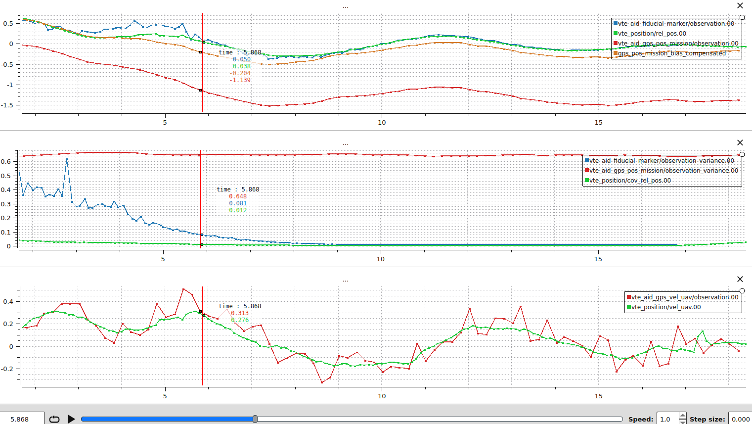
What this plot tells you:

1. Vision is the dominant source throughout the descent. The two observation variances never cross: vision is more precise than the mission GNSS at every altitude in this flight. This is intentional because the GPS module on the vehicle is not RTK-grade and the reported variance reflects that. If your receiver is more precise, retune VTE_GPS_P_NOISE so the floor does not throw away its confidence.
2. Higher altitudes have noisier vision. At the start of the descent vision is noisier and vte_position.rel_pos[0] deviates from individual vision samples. The vertical red line marks the moment vision becomes very precise. From there the filter locks onto vision.
3. A steady offset between the filter and the compensated GNSS is a tuning signal. During the last phase of the landing, a roughly 15 cm gap between vte_position.rel_pos[0] and gps_pos_mission_bias_compensated remains. If a comparable gap is persistent in your logs, the bias state can be too tight to absorb the slow drift. Loosen VTE_BIAS_UNC so the bias has more process noise, or lower VTE_GPS_P_NOISE so GNSS pushes the bias harder. Do not push either knob too far: a bias that moves too freely will drift when vision is lost, see Vision occlusion during descent.
4. End-of-flight vision loss. Vision stops detecting the target at the end of the trace and vte_position.cov_rel_pos starts to climb. The corrected GNSS still points to the pad thanks to the latest bias value, so the vehicle keeps tracking it.

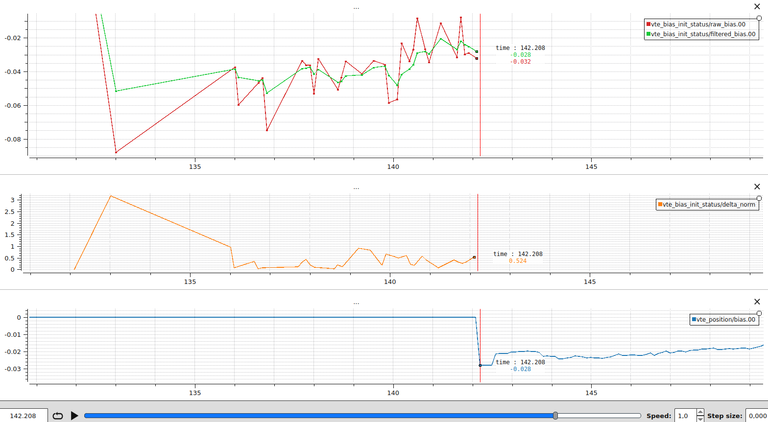
Initial bias averaging: Shows the GNSS/vision bias low-pass filter while the estimator is in the GNSS-first averaging phase. The plot was generated with VTE_BIA_AVG_TOUT=10s and VTE_BIA_AVG_THR=0.01 so the convergence threshold is never met and the full 10 s averaging window is exercised.

• Top row (raw vs filtered bias): vte_bias_init_status.raw_bias (per-axis raw GNSS minus vision delta) overlaid with vte_bias_init_status.filtered_bias. The filtered bias is the LPF output (tau = 0.3 s). It should track the average of the raw samples and settle to a steady value as more vision observations arrive.
• Second row (delta norm): vte_bias_init_status.delta_norm is the norm of consecutive raw-bias deltas which is the stability metric used by the convergence test. With VTE_BIA_AVG_THR=0.01 the filter would exit as soon as five consecutive deltas stay below 0.01 m and at least 2 * tau has passed. This threshold can be tuned based on the precision of the vision sensor.
• Third row (state activation): vte_position.bias jumps from zero to the activated bias once averaging completes. The reset uses r = pos_rel_gnss(t_vision) - b_filtered, b = b_filtered, so after activation vte_position.rel_pos aligns with the vision observation while vte_position.bias stores the GNSS offset.

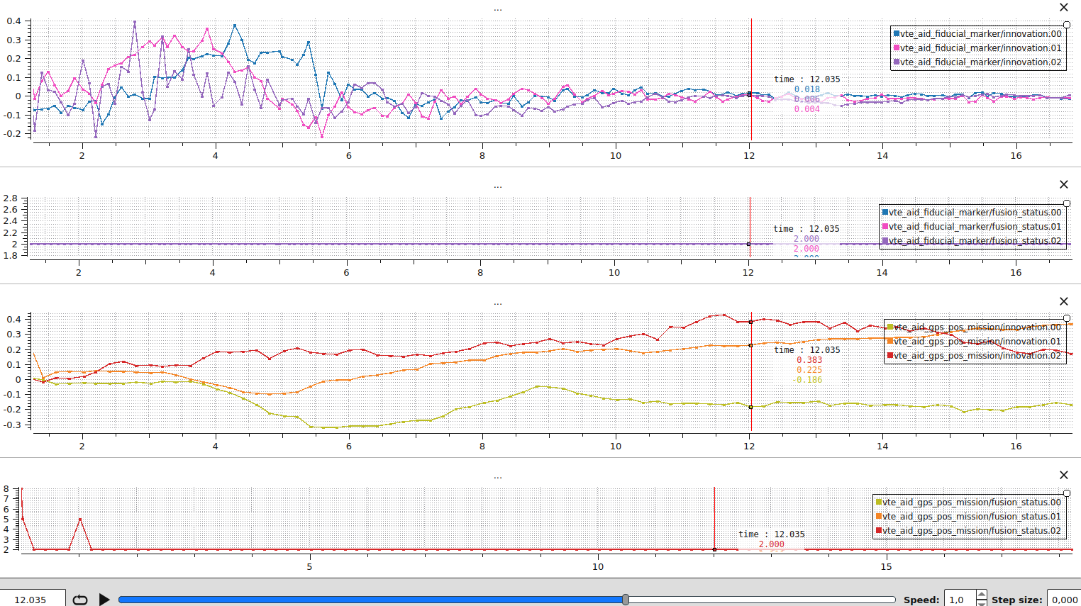
Innovation consistency: Confirms that every fused sensor produces zero-mean white-noise innovations. Generated from the same real precision-landing flight as the dashboard above, with vision and the mission landing waypoint as the absolute reference. The dashboard intentionally pairs a healthy aid source (vision) with a less well-tuned one (mission GNSS) so the two patterns can be compared side by side.

• Top row (vision innovations): vte_aid_fiducial_marker.innovation[0..2] on all three NED axes. The innovations look like white noise centred on zero, which is the healthy signature. They are slightly larger at higher altitudes where vision is noisier.
• Second row (vision fusion status): vte_aid_fiducial_marker.fusion_status[0..2] stays at 2 (STATUS_FUSED_OOSM), so every sample is fused via the OOSM history replay. The exact status code matters less than the fact that the sample is fused: STATUS_FUSED_CURRENT and STATUS_FUSED_OOSM are both healthy.
• Third row (mission GNSS innovations): vte_aid_gps_pos_mission.innovation[0..2]. The innovations are not zero-mean white noise. A persistent bias is visible at the vertical red line (about -0.18 m in North, +0.22 m in East, and +0.38 m in Down). The bias state is too tight to absorb the slow drift between the GNSS frame and the vision frame, so the residual ends up in the innovation. Loosen VTE_BIAS_UNC to let the bias track more of that drift, but only enough that the bias still stays stable when vision is lost (see Vision occlusion during descent).
• Bottom row (mission GNSS fusion status): vte_aid_gps_pos_mission.fusion_status[0..2] is mostly STATUS_FUSED_OOSM, so the GNSS variance is wide enough to absorb the biased innovation through the NIS gate. A short burst of STATUS_REJECT_TOO_OLD (status code 5) is also visible, meaning a GNSS sample arrived older than the OOSM buffer span (500 ms). To investigate, plot vte_aid_gps_pos_mission.time_since_meas_ms next (the OOSM under measurement delay dashboard is the right template).

Orientation filter: Validates that yaw aiding stays smooth yet responsive without making the drone oscillate. Generated from a real precision-landing flight. Enable the orientation filter with VTE_YAW_EN to log the same signals.

• Top row (yaw observation vs. state): vte_aid_ev_yaw.observation overlaid with vte_orientation.yaw. The state should track the slow trend of the observation without copying its high-frequency jitter.
• Second row (innovation, rad): vte_aid_ev_yaw.innovation should resemble white noise centred on zero.
• Third row (innovation, deg): same signal converted to degrees, which is the unit most users intuitively reason about when setting VTE_EVA_NOISE.
• Bottom row (test ratio): vte_aid_ev_yaw.test_ratio should stay below VTE_YAW_NIS_THRE.

If the yaw state follows the observation noise, the solution is the same as for position: raise the observation floor or stiffen the prediction. See When the state follows per-sample jitter.

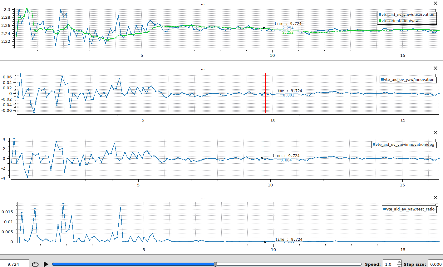
Case study: yaw oscillation. The plot above was generated with VTE_EVA_NOISE at 4 deg (about 0.07 rad) and VTE_YAW_ACC_UNC at 0.004, both current defaults. With more aggressive values (0.05 rad / 0.04) the filter jumped to follow every yaw observation, the controller chased the resulting setpoint changes, and the drone visibly oscillated. The oscillation itself then degraded the next vision samples (motion blur and larger lever-arm effects make yaw harder to estimate), feeding the loop. Trusting the process model more (smaller VTE_YAW_ACC_UNC) and the observations less (larger VTE_EVA_NOISE) breaks that loop: the state stays close to the underlying yaw trend, the drone holds steady, and the observations themselves become cleaner.

Click to view Out-of-Sequence Measurements (OOSM) plots

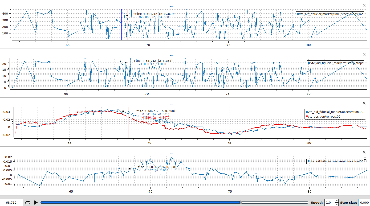
OOSM under measurement delay: Shows that delayed measurements are still consumed correctly thanks to the OOSM history replay. The plot was generated by delaying each simulated measurement by a uniform random value in [0, 500] ms before reaching the autopilot.

• Top two rows (measurement latency): vte_aid_fiducial_marker.time_since_meas_ms and vte_position.history_steps. With a 0-500 ms delay we observe time_since_meas_ms ranging up to ~450 ms and history_steps proportional to it (history_steps ≈ time_since_meas_ms / 20, at most 24 with the 25-snapshot buffer).
• Third row (raw vs processed observation): vte_position.rel_pos overlaid with vte_aid_fiducial_marker.observation. The processed observation lags the live state by roughly the measurement delay. The OOSM allows fusing old data without forcing the live state to wait for it.
• Fourth row (innovation): vte_aid_fiducial_marker.innovation[0] stays close to zero. The innovation is computed against the predicted state at t_meas, not against the current live state, so the latency cancels out.

A concrete sample from this run: at $t=68.712$ s (vertical red line) the live state is vte_position.rel_pos[0] = 0.026 m and the measurement that just arrived is vte_aid_fiducial_marker.observation[0] = 0.041 m, with time_since_meas_ms = 368 ms and history_steps = 21. Looking 368 ms back into the history at $t=68.344$ s (blue vertical line), vte_position.rel_pos[0] = 0.034 m. The OOSM innovation is computed against that historic prediction, giving $0.041-0.034=0.007$ m, which matches vte_aid_fiducial_marker.innovation[0] = 0.007 m. Without OOSM the filter would compare the delayed measurement against the live state and produce $|0.026-0.041|=0.015$ m instead which is roughly twice as large. Under fast dynamics this kind of latency-induced error grows quickly and can repeatedly fail the chi-squared gate or pull the state in the wrong direction causing overshoots.

Click to view filter robustness plots

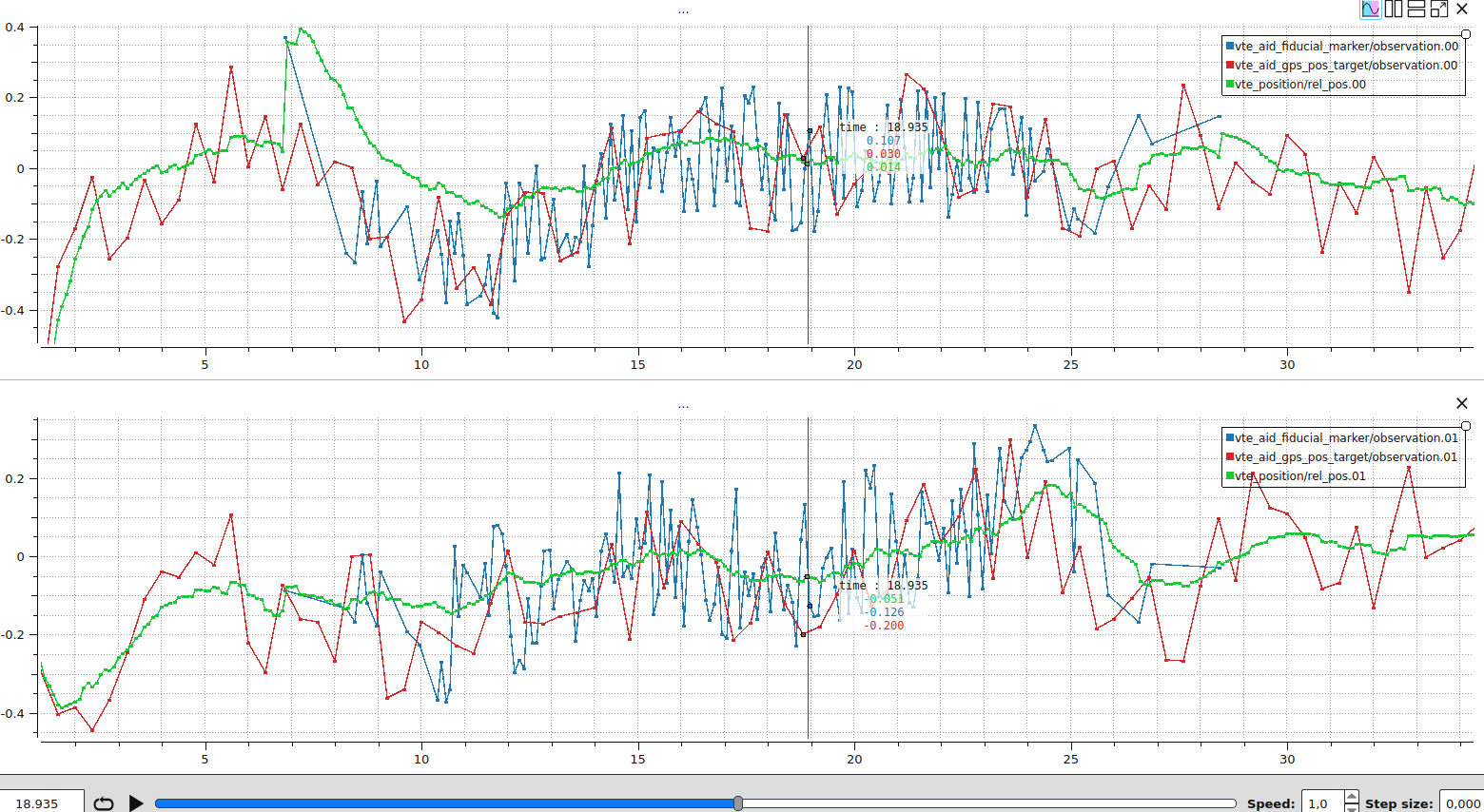
Smoothing through bounded noise: When the filter is well tuned, the state stays smooth even when individual observations are noisy. The plot was generated by adding uniform random noise in the range $[-0.20,+0.20]$ m to both the vision (vte_aid_fiducial_marker.observation) and target-GNSS (vte_aid_gps_pos_target.observation) position observations on the x, y, z axes. The injected noise stays within the NIS gate, so every sample is fused.

• Top row (x axis): vte_aid_fiducial_marker.observation[0] and vte_aid_gps_pos_target.observation[0] are visibly noisy, but vte_position.rel_pos[0] follows the underlying trend smoothly.
• Bottom row (y axis): same behaviour on the lateral axis.

The smoothness is the Kalman filter doing its job: each sample only contributes a fraction of its innovation to the state, weighted by the ratio of the predicted state variance to the observation variance. As long as the noise stays inside the NIS gate, no rejection happens and the per-sample jitter averages out across many fusions. If the state in your own logs follows the jitter instead of the trend, see When the state follows per-sample jitter for the tuning recipe.

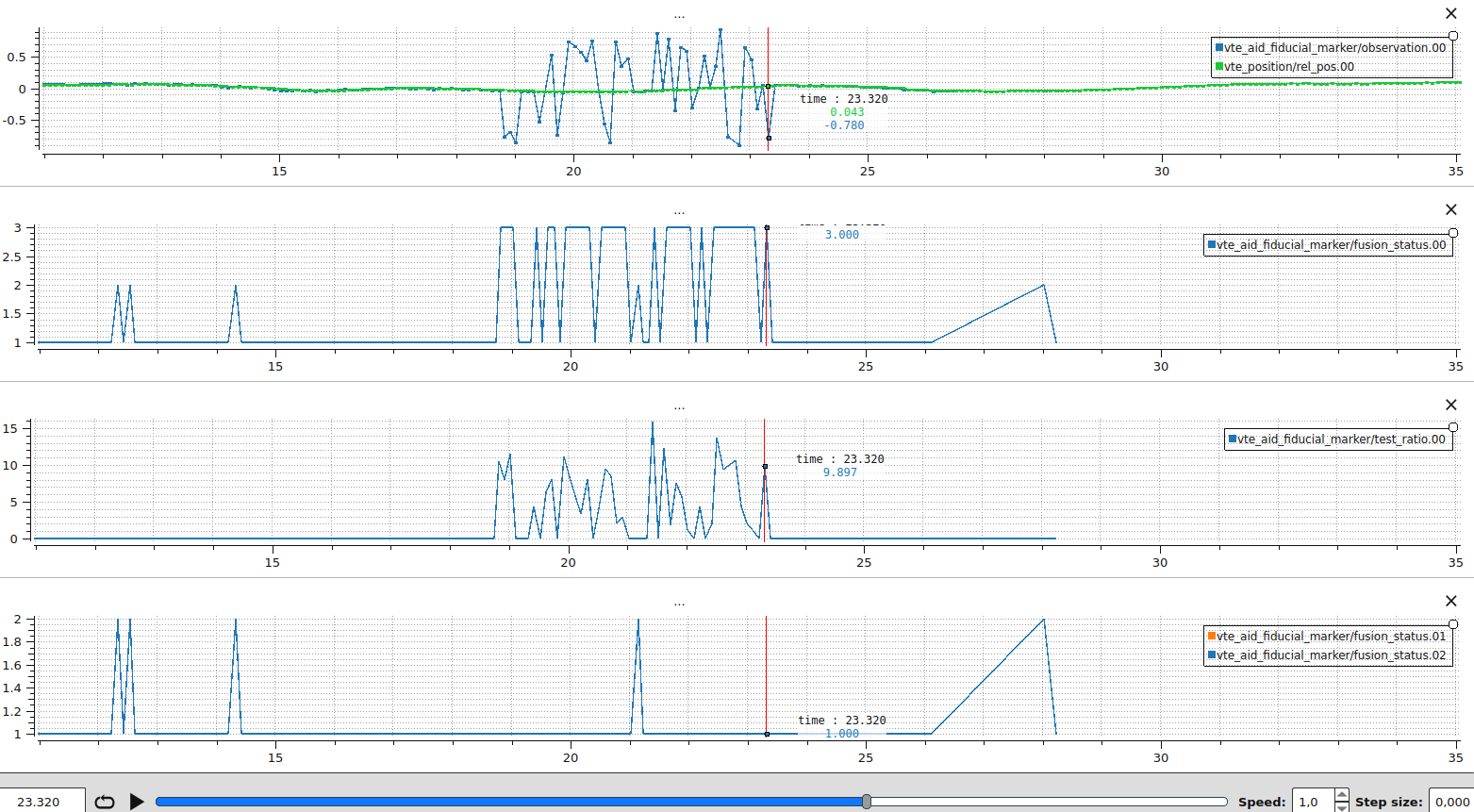
Rejecting a corrupted measurement: Demonstrates how the estimator rejects a faulty measurement. The plot was obtained by injecting during 6 seconds an additive bias uniformly sampled between -1 and 1 metre on the x-axis vision observation, while leaving the other axis untouched. The healthy axes keep fusing as expected, while the corrupted axis repeatedly fails the NIS gate, which keeps the state from chasing the outliers.

• Top row (x observation): vte_position.rel_pos[0] follows vte_aid_fiducial_marker.observation[0] until the measurements are altered, at which point it does not follow the biased measurements.
• Second row (x fusion status): vte_aid_fiducial_marker.fusion_status[0] flips to STATUS_REJECT_NIS whenever the observation disagrees with the filter prediction, confirming that the chi-squared gate is doing its job.
• Third row (x test ratio): vte_aid_fiducial_marker.test_ratio[1] spikes and breaches VTE_POS_NIS_THRE for the biased measurements.
• Bottom row (y, z fusion status): vte_aid_fiducial_marker.fusion_status stays at 1: STATUS_FUSED_CURRENT or 2: STATUS_FUSED_OOSM in the y and z direction.

What to do when you see this pattern in your own logs:

1. Confirm that the rejection actually corresponds to a corrupted measurement and not a healthy sample being thrown out by an overly tight gate. Compare the raw sensor topic (e.g. fiducial_marker_pos_report) with vte_aid_fiducial_marker.observation to be sure the input itself is bad rather than a frame transform or timestamp issue.
2. If the rejections are legitimate (the data really is corrupted), no parameter change is needed: the NIS gate is doing its job. Investigate the upstream sensor instead (camera exposure, marker visibility, attitude alignment).
3. If healthy samples are being rejected, the observation variance is the first thing to revisit. As detailed in the troubleshooting checklist row on Frequent innovation rejections, an under-reported variance causes the NIS gate to fire on small innovations. Raise VTE_EVP_NOISE (or VTE_GPS_P_NOISE for GNSS) so the floor matches the actual sensor accuracy.
4. If both the upstream sensor and the variance look correct but legitimate outliers are still slipping through, loosen the gate slightly with VTE_POS_NIS_THRE (defaults to 3.84, i.e. a 5% false-rejection rate). Larger values are more permissive, smaller values reject more aggressively.

Vision dropout behaviour: Illustrates what happens when vision is the only relative-position source and the marker is temporarily lost, and why fusing the vehicle GNSS velocity matters in practice.

Both plots come from the same SITL scenario with a static target: the filter is well converged on vision, vision drops out for several seconds, then comes back. The only difference between the two runs is whether VTE_AID_MASK bit 1 (vehicle GNSS velocity) is enabled.

To make the full dropout visible, VTE_BTOUT was raised to 10 s for these runs (default 3 s) so the filter keeps predicting the state instead of resetting early. On both plots the vertical blue line marks the moment vision is lost, and the vertical red line marks the estimator timeout 10 s later, when VTE_BTOUT expires and the filter is reset.

This is a structural property of the filter, not a tuning issue. See Filter observability for the underlying reason: vision never touches the $v^{uav}$ state directly, so any residual in $v^{uav}$ integrates straight into vte_position.rel_pos once vision is gone.

Plot 1, vision only: VTE_AID_MASK = vision only (bit 2).

• Top row (relative position): vte_position.rel_pos[0] overlaid with vte_aid_fiducial_marker.observation[0]. The state stays close to the last vision sample for roughly 3 seconds after the dropout (the time it takes the residual $v^{uav}$ to integrate to a visible offset), then drifts by about 60 cm over the next 7 seconds. When vision returns, the state snaps back by ~60 cm in a single innovation, which is the accumulated drift.
• Bottom row (UAV velocity): vte_position.vel_uav[0], vehicle_local_position.vx, and sensor_gnss.vel_north. The three traces agree while vision is fused. As soon as vision drops, the filter estimate diverges by about 0.1 m/s from the EKF2 and GNSS references. That ~0.1 m/s gap over 7 seconds is the position drift observed in the top row.

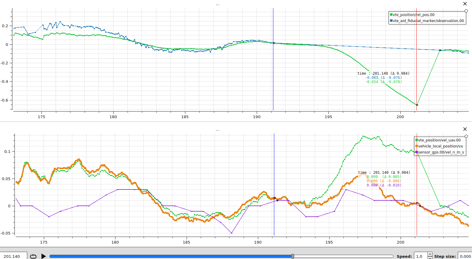
Plot 2, vision and vehicle GNSS velocity: Same scenario, with VTE_AID_MASK bit 1 enabled. Vehicle GNSS velocity is now fused as $z=v^{uav}$, which gives the velocity state a direct observation independent of vision.

• Top row (relative position): vte_position.rel_pos[0] properly follows the expected trend through the dropout. The correction on vision recovery is small (in this run, from 0.26 m to 0.24 m, i.e. 2 cm), which is within the vision noise level rather than a real drift.
• Bottom row (UAV velocity): vte_position.vel_uav[0] now tracks vehicle_local_position.vx and sensor_gnss.vel_north for the full dropout, because GNSS velocity continues to constrain the state when no vision sample is available.

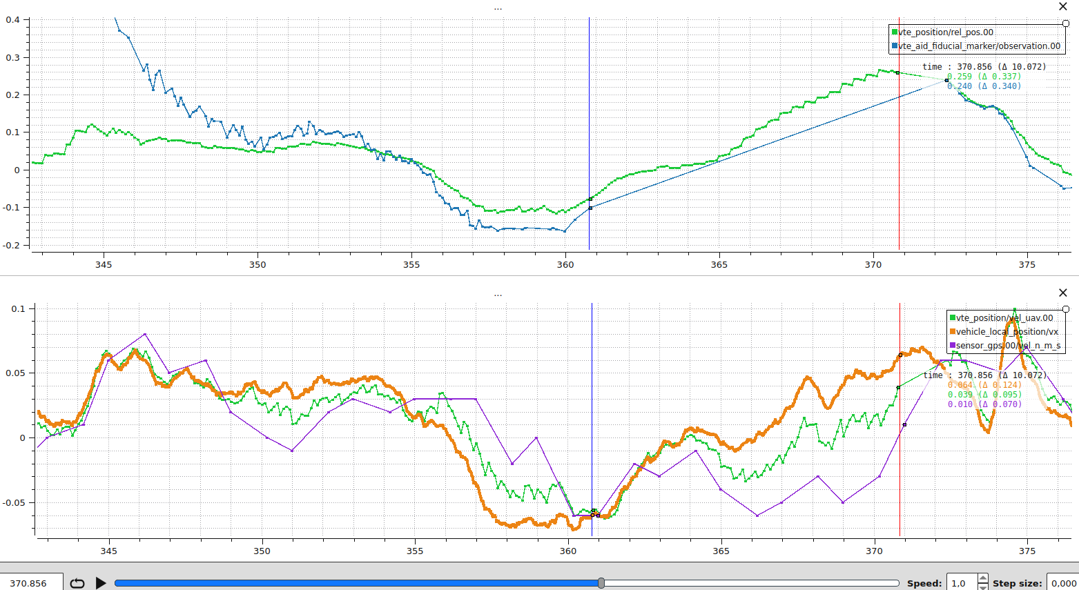
What to take away from this comparison:

1. With vision alone, the vehicle velocity state is only weakly observable, so the filter cannot estimate cleanly through gaps in vision. Any additional source that touches the velocity state directly substantially extends how long the filter remains accurate without a vision sample.
2. The size of the relative-position jump on vision recovery is a useful diagnostic on its own: a large jump means the velocity state had drifted during the gap, not that the recovered vision sample is wrong.

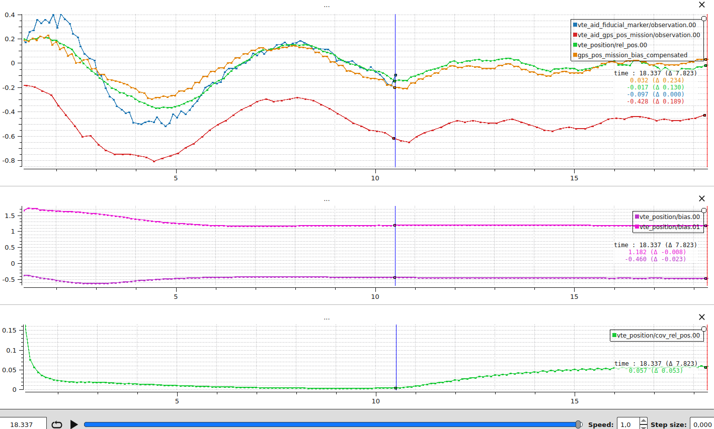
Vision occlusion during descent (real flight): Demonstrates the central motivation behind multi-sensor fusion. Once the bias between the absolute frame (here the mission landing waypoint) and the vision frame is estimated, the corrected GNSS observation still points at the pad after vision drops out, so the vehicle still lands precisely. Generated by removing the vision fusion 5 m above the target during a real precision-landing flight. The drone landed at the center of the target despite the vision loss.

The vertical blue line marks the moment vision is stopped, and the vertical red line marks touchdown.

• Top row (relative position and bias-compensated GNSS): vte_aid_fiducial_marker.observation[0], vte_aid_gps_pos_mission.observation[0], vte_position.rel_pos[0], and the custom trace gps_pos_mission_bias_compensated = vte_aid_gps_pos_mission.observation[0] - vte_position.bias[0].
• Middle row (bias estimates): vte_position.bias[0] and vte_position.bias[1]. The bias converges in roughly 6 seconds as the drone descends and vision becomes more precise. Between the blue and red lines (8 seconds without vision), the deltas are about $-0.023$ m on x and $-0.008$ m on y, so the bias stays effectively stable. By touchdown, the bias settles at about $-0.46$ m on x (north) and $+1.18$ m on y (east). Without bias compensation the drone would have touched down 1.18 m east of the pad.
• Bottom row (relative position covariance): vte_position.cov_rel_pos[0]. The variance climbs by about 0.053 m² once vision is lost, corresponding to a 1-sigma growth of $\sqrt{0.053}\approx 0.23$ m. This is the filter reporting that the relative position is now less certain because no vision sample is constraining it.

This is the case multi-sensor fusion was designed for. The mission landing waypoint reports the pad position with a metre-scale offset (the bias) that vision corrects. Once the bias is observed, the corrected GNSS effectively becomes a second relative-position sensor for the remaining descent, including any segment where the marker temporarily disappears (motion blur, partial occlusion, or the marker leaving the camera field of view because it is too large at low altitude). This is particularly important for large targets where the marker is expected to leave the camera frame in the final metres of descent.

What to watch in your own logs:

• The bias must already be settled before vision drops out. If your dropout test shows the bias still moving when vision is lost, lower VTE_BIAS_UNC.
• The post-dropout bias drift gives a direct read on how aggressively the bias is tuned. The deltas above (a few centimetres over 8 seconds) match a well-tuned filter. Larger drift means VTE_BIAS_UNC is too loose. The filter overfit the bias to recent vision and now lets it walk away when vision is gone.

Click to view Precision Landing on a static target plot

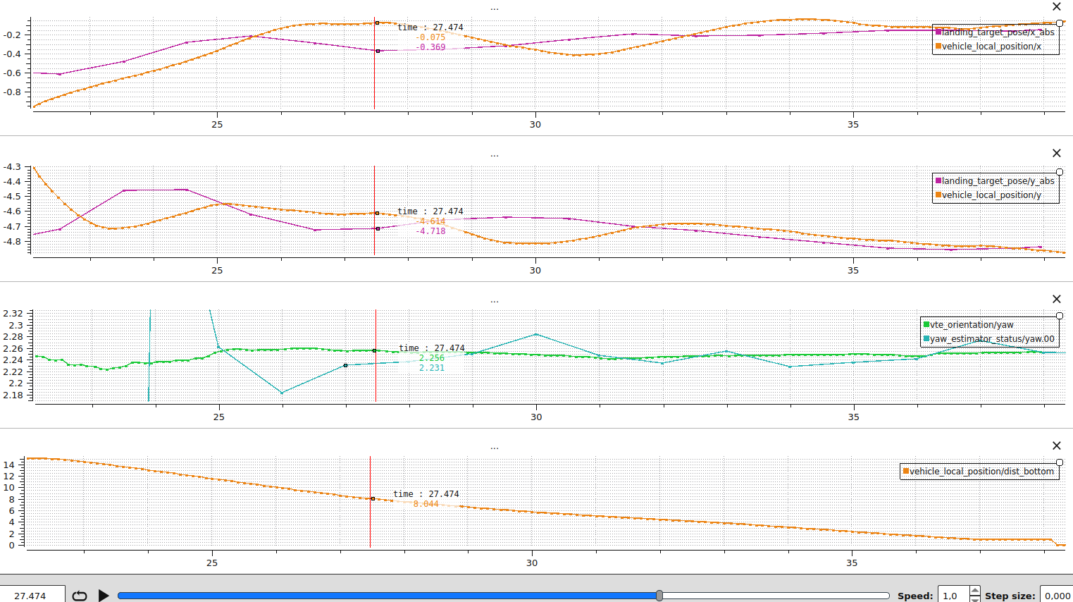
Precision landing alignment: Compares the precision-landing target with the vehicle position to confirm that the vehicle is actually navigating toward the target. Generated from a real precision-landing flight.

landing_target_pose.x_abs and landing_target_pose.y_abs are expressed in the local NED frame, which is fixed relative to the EKF2 origin. For a static target both values should stay roughly constant for the duration of the approach. The estimator can refine the target position as new observations arrive, but big jumps or steady drift in this signal indicate noisy observations or an estimator that is following them too aggressively. If you see this, When the state follows per-sample jitter lists the right knobs.

The plot is also useful for catching misconfigurations, for example PLD_YAW_EN disabled when yaw alignment is expected. If the controller struggles to follow even when the target signal is clean, review the multicopter position tuning guide.

• Top row (north alignment): landing_target_pose.x_abs against vehicle_local_position.x. The curves should overlay once precision landing is triggered.
• Second row (east alignment): landing_target_pose.y_abs against vehicle_local_position.y, same as north.
• Third row (yaw alignment): vte_orientation.yaw should remain steady while trajectory_setpoint.yaw tracks it when PLD_YAW_EN is enabled.
• Bottom row (descent context): vehicle_local_position.dist_bottom shows when the final approach begins and how high above the pad the precision-landing alignment converged. A higher convergence altitude is better.

Click to view Moving Target plot

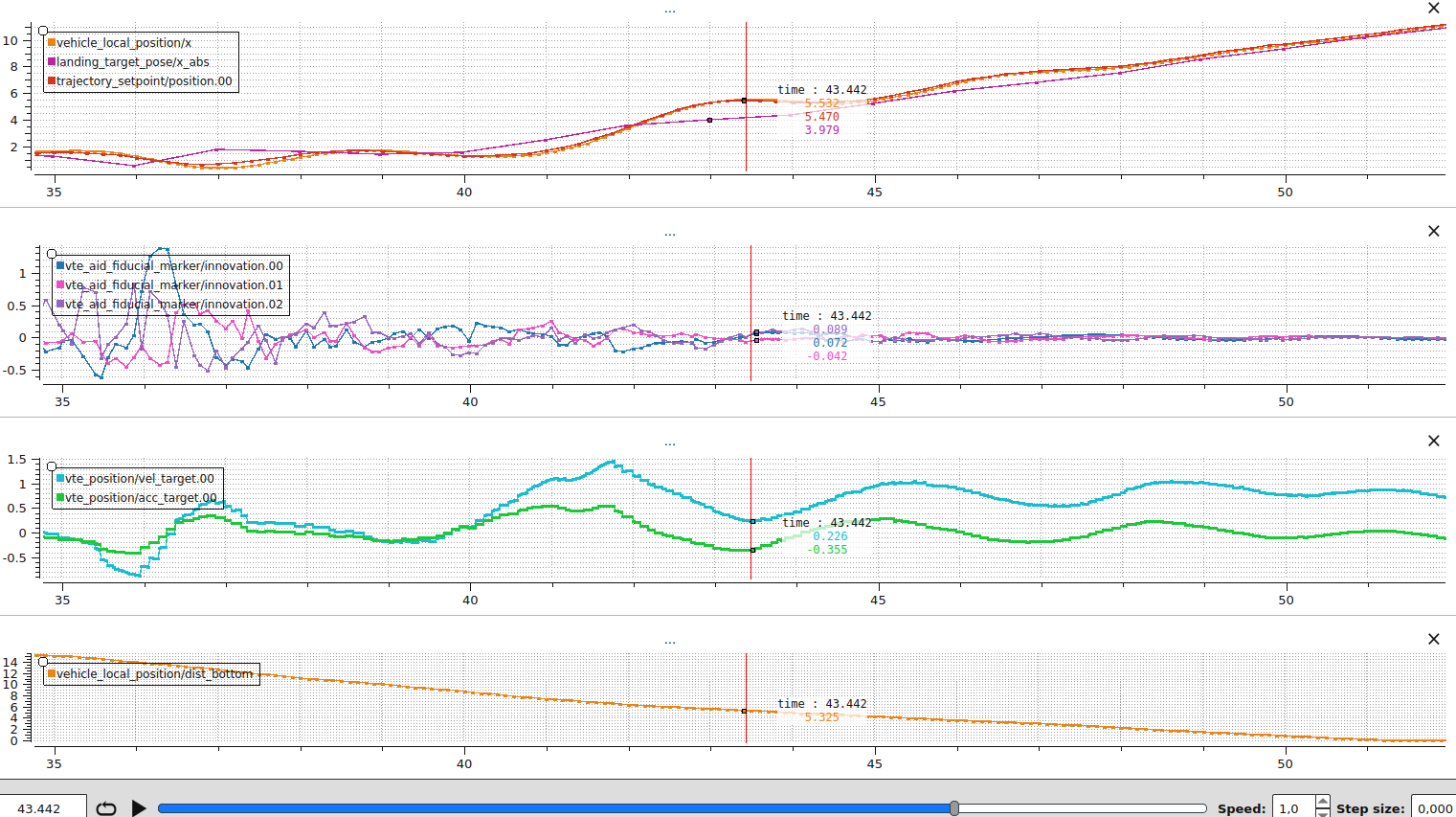
Moving target precision landing: Shows how the precision-landing controller projects the setpoint ahead of a moving target, how the lead converges onto the target as altitude drops, and how the moving-target states behave during the descent. Generated from a real flight with a camera publishing target estimates at 10 Hz at 640×480 resolution. The firmware was built with CONFIG_VTEST_MOVING=y.

• Top row (axis along which the target moves): vehicle_local_position.x, landing_target_pose.x_abs, and trajectory_setpoint.position[0]. The trajectory setpoint sits ahead of the estimated target position for most of the descent: that is the PLD_MOVING_T_MAX lookahead leading the vehicle toward where the target will be at touchdown. As altitude drops, the lookahead converges toward PLD_MOVING_T_MIN, the gap between setpoint and target closes, and the vehicle lands on the moving target rather than where it was at the start of the approach.
• Second row (vision innovations): vte_aid_fiducial_marker.innovation[0..2] on all three NED axes. They look like white noise centred on zero, which means the filter dynamics match the marker observations even as the target moves.
• Third row (moving-target states): vte_position.vel_target and vte_position.acc_target. These states only exist in the moving-target build and can be compared to the expected target velocity and acceleration.
• Bottom row (descent context): vehicle_local_position.dist_bottom shows the distance to the ground and indicates the phase of the landing.

What to take away:

• Add more sensors when you can. With vision only, the mission must end up somewhere the target is visible because the filter has no other observation of the target position. Adding a target GNSS receiver gives the filter an absolute reference even before vision detects the marker: the filter converges faster, the vehicle can fly to a moving target before it is in view, and the risk of missing the target is reduced. Any offset between the receiver and the marker is estimated by the bias state.
• Add a direct target-velocity observation when you can. Target GNSS velocity (VTE_AID_MASK bit 4) is the only measurement that constrains $v^t$ directly, and without it the precision-landing lookahead becomes noisier. See Filter observability for why a direct velocity observation matters.
• Publish target estimates at a high rate. With a 10 Hz camera the prediction has up to 100 ms of unconstrained motion between samples. Raising the rate shrinks the predicted variance growth between fusions, makes the precision-landing setpoint smoother, and keeps vte_aid_fiducial_marker.innovation closer to zero through the descent.

Development and Debugging Tips

A few tips to make iteration on real hardware and SITL easier.

• To print PX4_DEBUG statements from the module, launch SITL with PX4_LOG_LEVEL=debug (for example, PX4_LOG_LEVEL=debug make px4_sitl_visionTargetEst). On hardware builds, compile with the debug configuration or enable the console log level before running tests so the additional diagnostics appear on the shell.
• Keep the estimator alive on the bench by setting VTE_TASK_MASK=3. The debug bit enables the continuous update of the position and orientation estimators (if enabled via VTE_YAW_EN and VTE_POS_EN).
• Use vision_target_estimator status for the compact health summary. Inspect state values with listener vte_position and listener vte_orientation, published output with listener landing_target_pose, bias averaging with listener vte_bias_init_status, innovations with listener vte_aid_fiducial_marker (or the relevant vte_aid_*), and prediction inputs with listener vte_input 5.

Click to view the guide on SITL Simulation Pipeline

The Gazebo Classic SITL setup produces both VTE inputs (fiducial_marker_pos_report and target_gnss) end-to-end, so the filter can be tested without real hardware. This is also where you should inject extra noise or latency to stress-test the filter.

The pipeline has four stages:

1. Aruco marker detection: arucoMarkerPlugin (Tools/simulation/gazebo-classic/sitl_gazebo-classic/src/gazebo_aruco_plugin.cpp) runs on the simulated camera, detects the marker, and publishes a TargetRelative Gazebo message. The reported standard deviations are hard-coded in OnNewFrame() (set_std_x, set_std_y, set_std_z, set_yaw_std). Change them there to make the simulated vision report noisier or cleaner. Marker visibility is controlled by Tools/simulation/gazebo-classic/sitl_gazebo-classic/models/land_pad/land_pad.sdf: the <visual><box><size> element sets the rendered Aruco square (the <collision> size is independent and just controls the physical pad). The <pose> element on the <model name="land_pad"> block places the pad in the world. Its last value is the pad yaw in radians (for example <pose>0.0 0.0 0.06 0 0 0.7</pose> rotates the pad by 0.7 rad, about 40 deg), which is the easiest way to exercise the orientation filter in SITL.
2. Target GPS: the gps_target model included from land_pad.sdf runs the standard Gazebo GPS plugin. Tune the noise floors directly in Tools/simulation/gazebo-classic/sitl_gazebo-classic/models/gps/gps.sdf (the <noise> blocks for horizontal/vertical position and velocity).
3. Mavlink bridge: gazebo_mavlink_interface.cpp connects the two plugins to the autopilot. targetRelativeCallback() packs the marker into a TARGET_RELATIVE mavlink message, and TargetGpsCallback() packs the GPS sample into TARGET_ABSOLUTE.
4. PX4 side: SimulatorMavlink::handle_message_target_relative() and handle_message_target_absolute() decode the mavlink messages back into fiducial_marker_pos_report and target_gnss (or directly into landing_target_pose when VTE_EN=0). From there the filter sees exactly the same topics it would on real hardware, so anything you tune at the sensor level reproduces faithfully end to end.

Click to view the guide on adding new measurement sources

To integrate a new sensor:

1. Define a uORB message that carries the measurement in either the vehicle body frame or NED, complete with variance estimates and timestamps.
2. Extend the fusion mask: add a bit to SensorFusionMaskU (src/modules/vision_target_estimator/common.h) and update the parameter definition for VTE_AID_MASK (see also sensor fusion selection) in vision_target_estimator_params.yaml.
3. Augment observation enums: append the new entry to the relevant ObsType enum (VTEPosition.h or VTEOrientation.h), update ObsValidMaskU, and update helper functions such as hasNewNonGpsPositionSensorData() and selectInitialPosition() if the measurement can provide a relative position.
4. Subscribe and validate: add a uORB::Subscription to the filter, check for finite values, move small future offsets to the current time with alignFutureSampleTime(), and reject samples that are too old isMeasUpdated or further in the future before marking the observation valid.
5. Implement the handler in processObservations(). Convert the measurement into NED coordinates, populate TargetObs::meas_xyz, meas_unc_xyz, and the observation Jacobian (meas_h_xyz or meas_h_theta), and set the fusion-mask flag only after the data passes validation.
6. Provide tunable noise: declare a parameter (e.g. VTE_<SENSOR>_NOISE) and clamp it with kMinObservationNoise so the estimator never believes a measurement is perfect.
7. Log the innovations: add a publication member and ORB topic (see vte_aid_fiducial_marker for reference) so that logs include the innovation, variance, and fusion_status outcome for the new sensor. Use the FusionResult returned by the filter to populate fusion_status so successes and rejections share the same status enum as the existing sources.
8. Exercise SITL: update the Gazebo (or other) simulation so that replay tests produce the new measurement. This keeps CI coverage intact and provides a reference data set for tuning.
9. Document the workflow: update this deep dive and any setup how-tos so users know how to enable the new bit, calibrate the sensor, and interpret its logs.

WARNING

Timeout policy: Every measurement must be time-aligned and checked so that stale data never reaches the update step. Reject samples older than VTE_M_REC_TOUT (isMeasRecent(hrt_abstime ts)) and check time_since_meas_ms (and fusion_status for STATUS_REJECT_TOO_OLD / STATUS_REJECT_TOO_NEW) on the new vte_aid_* topic to confirm the sensor fits inside the estimator deadlines. If observations are stored in cache, invalidate it inside checkMeasurementInputs when older than VTE_M_UPD_TOUT (isMeasUpdated(hrt_abstime ts)).

Click to view the guide on adding new tasks

Add a new VteTask when the estimator should only run during a particular mission phase or flight-mode behaviour, or when that behaviour needs its own subscriptions, cached state, or completion logic. Do not put that state back into VisionTargetEst. The whole point of the task layer is to keep the scheduler generic.

Use this checklist:

1. Reserve a task-mask bit: add the bit in task_bits (tasks/VteTask.h). Those constants are the code-level source of truth for VTE_TASK_MASK. Then update vision_target_estimator_params.yaml and the VTE_TASK_MASK documentation so users can enable the new task.
2. Create a task class: add a new file under src/modules/vision_target_estimator/tasks/ and derive it from VteTask. Put all task-specific subscriptions and status flags in that class.
3. Implement the interface deliberately: maskBit() and name() identify the task, pollStatus() refreshes external state, isReady() exposes level-triggered readiness, and isComplete() reports self-termination. Use onActivate() for one-shot state resets on task entry, and onPosEstStart() only when the position filter needs task-specific seeding such as a cached mission waypoint.
4. Keep side effects out of readiness checks: pollStatus() and isReady() are called every scheduler cycle while the task bit is enabled. They should be cheap. Transition-only work belongs in onActivate().
5. Register the task by priority: add the task instance to VisionTargetEst and place it in _task_registry in descending priority order. If multiple bits are enabled at the same time, the first ready task wins.
6. Test lifecycle and cache behaviour: extend TEST_VTE_VisionTargetEst.cpp with coverage for task activation completion, repeated starts, and any cached mission/context data that must survive estimator restarts within the same task.
7. Document the operational meaning: update the overview page, this deep dive, and any feature-specific docs so users understand when the new task is active and which VTE_TASK_MASK bit selects it.

Click to view the guide on SymForce-generated derivations

The Kalman-filter math is not written by hand. The symbolic state, prediction model, and covariance update are defined in Python and expanded into C++ by SymForce, so the C++ that runs on the autopilot always matches the model defined in derivation.py.

Source files (Python):

• src/modules/vision_target_estimator/Position/vtest_derivation/derivation.py for the position filter.
• src/modules/vision_target_estimator/Orientation/vtest_derivation/derivation.py for the yaw filter.

Generated outputs (C++ headers) used at runtime:

Filter	Generated headers
Position	state.h, predictState.h, predictCov.h, computeInnovCov.h, applyCorrection.h
Orientation	predictState.h, predictCov.h (innovation computation and correction stay hand-written in Orientation/KF_orientation.cpp so yaw angles can be wrapped to $[-\pi ,\pi ]$)

Build-time behaviour:

• By default, CMake copies the committed pre-generated headers from Position/vtest_derivation/generated/ into the build tree under build/<target>/src/modules/vision_target_estimator/vtest_derivation/generated/, and likewise for orientation. No SymForce install is required for the static build.
• CONFIG_VTEST_MOVING=y automatically sets VTEST_SYMFORCE_GEN=ON and requires SymForce in the Python environment so the 5-state moving-target headers are produced.
• Setting -DVTEST_SYMFORCE_GEN=ON manually regenerates both filters at configure time.

The generated files are included from the build directory and must never be edited by hand. To change the model, edit derivation.py and regenerate.

Regenerating the symbolic model

1. Configure CMake with -DVTEST_SYMFORCE_GEN=ON (automatic when CONFIG_VTEST_MOVING=y) and ensure SymForce is available in the Python environment.
2. Reconfigure with cmake --fresh ... so the custom command in src/modules/vision_target_estimator/CMakeLists.txt runs. The outputs land in build/<target>/src/modules/vision_target_estimator/vtest_derivation/generated/ (position) and .../vte_orientation_derivation/generated/ (orientation).
3. To refresh the committed reference files, add -DVTEST_UPDATE_COMMITTED_DERIVATION=ON and commit the regenerated files in Position/vtest_derivation/generated*/ once vetted.

If the build fails during regeneration, inspect the CMake output for the SymForce invocation and rerun it manually inside Position/vtest_derivation/ to catch Python errors. After regenerating, rebuild the module to ensure the Jacobians and code stay in sync.

Runtime Performance on Hardware

Read the estimator's elapsed-time counters from the shell:

perf | grep "VTE"

Counter	What It Measures
VTE cycle	Input handling and eligible position/yaw updates in updateEstimators().
VTE cycle pos	One position update, including input preparation and vte_input publication.
VTE cycle yaw	One orientation update.
VTE prediction	One prediction across all three position axes.
VTE update	Fusion of all position observations of one cycle, across the three axes.
VTE fusion	Fusing one cycle's observations on one position axis: at most one history replay.

These counters overlap; do not add their elapsed times to estimate CPU usage. Reset them with perf reset after warmup, and use top to measure the wq:vte CPU share. Replay cost increases with measurement delay and the number of later stored observations (see OOSM Implementation). Check the aid-source fusion_status fields alongside timing to confirm that observations are being fused.

Pixhawk 6C Reference Measurements

Measurements from 18 October 2026 used disarmed SIH with a stationary target and yaw estimation enabled. Vision was injected at 100 Hz and target GNSS at 50 Hz; native UAV GNSS ran at approximately 8 Hz. The moving-model trials enabled target GNSS position and velocity aiding. Actual estimator updates ran at approximately 43 to 44 Hz. Delayed inputs had 460 ms added to their capture age; native UAV GNSS had no added delay.

Model / Inputs	Mean Position Update, µs	Largest Observed, µs	VTE CPU
Static, fresh inputs	71.5	301	0.67%
Static, fresh vision and delayed target GNSS	327.1	570	1.72%
Static, delayed vision and target GNSS	427.0	667	2.28%
Moving, fresh inputs	117.8	813	0.87%
Moving, fresh vision and delayed target GNSS	1,437.3	1,867	6.06%

Each row summarises three 30-second trials; CPU includes position and yaw work, sampled in three approximately 1.2-second top windows per trial. Fresh inputs have no added delay, but transport and scheduling can still move them across the 20 ms OOSM threshold. These numbers predate the shared replay: rows with two delayed observations per cycle (delayed vision and target GNSS, or moving-mode target GNSS position and velocity) replayed the window twice per axis. These are reference measurements, not worst-case timing limits; measure your own board with its expected source rates and delays.

Unit Test Suites

The module contains unit tests that cover the Kalman math, the per-filter module logic, and the OOSM history buffer.

• TEST_VTE_KF_position: Kalman filter math for the position state (prediction, NIS gating, bias-aware H, OOSM gold standard). Static model (state size 3) by default, moving-target tests (state size 5) build only when CONFIG_VTEST_MOVING is enabled.
• TEST_VTE_KF_orientation: Kalman filter math for yaw/yaw-rate (wrap logic, process noise, dt edge cases, covariance symmetry).
• TEST_VTE_VTEPosition: Module logic for vision/GNSS fusion, offsets, interpolation, ordering, and uORB innovation topics (static + moving gated by CONFIG_VTEST_MOVING).
• TEST_VTE_VTEOrientation: Module logic for yaw fusion, noise models, resets, and OOSM handling.
• TEST_VTE_VTEOosm: Generic OOSM manager behaviour.

Run locally:

make tests TESTFILTER=TEST_VTE*